Posted: 08/24/21

Due: 09/03/21, 11:55PM

1Difference equations

1.1Mathematics of difference equations

1.2Fibonacci population model

In 1202 Fibonacci introduced a model of population growth based on discrete time reproduction with death or infertility.

1.2.1Hypotheses

The formal assumptions within the Fibonacci popoulation model are:

1. Count rabbit pairs, denote by $F$ one male and one female;

2. Assume rabbit pairs do not die;

3. Assume each pair reproduces in a constant time interval of one month;

4. Assume one unit of time from birth to fertility;

5. Assume each rabbit pair reproduces exactly one new rabbit pair;

6. Assume all rabits pairs are fertile.

Denote time by $n\in \mathbb{N}$, and let $F_n$ denote the number of pairs at time $n$.

1.2.2Mathematical formulation

The Fibonacci model leads to the relation

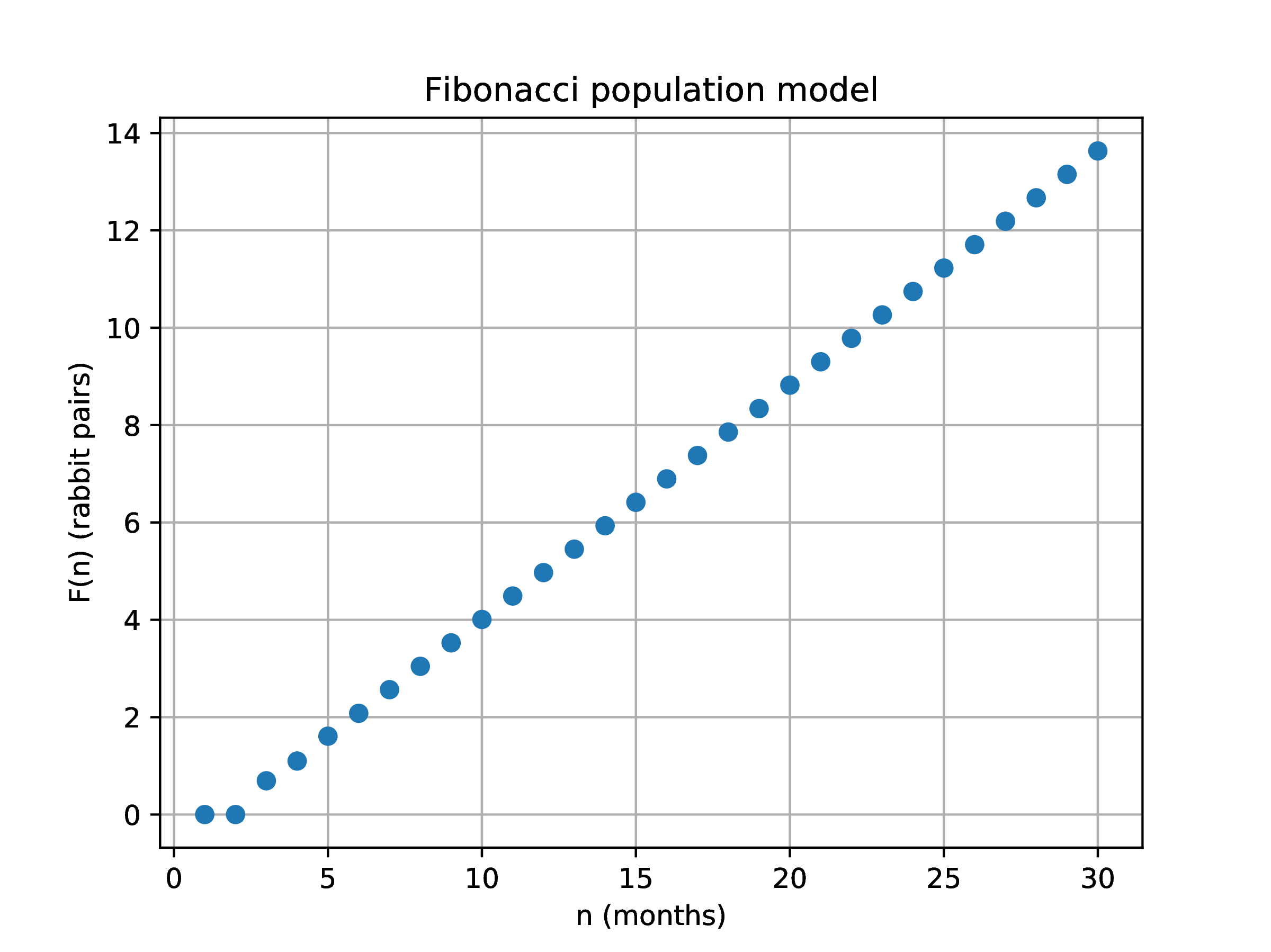
with initial conditions $F_0=0$, $F_1=1$. The model exhibits exponential growth as shown in Fig. 1

∴ 

function F(n)
  if ((typeof(n)==Int64) && (n>=0))
    if (n<2) 
       return n
    end
    return F(n-1)+F(n-2)
  else
    print("Invalid argument\n")
  end
end

1.2.3Direct computation

$•$

Figure 1. Logarithmic representation of Fibonacci rabbit pair growth.

∴	N=30; n=0:N; Fn=F.(n); clf(); plot(n,log.(Fn),"o");

∴	xlabel("n (months)"); ylabel("F(n) (rabbit pairs)");

∴	title("Fibonacci population model"); grid("on");

∴	savefig(homedir() * "/courses/MATH089/images/Fibonacci.eps")

∴

1.2.4Comparison of direct computation to analytical solution

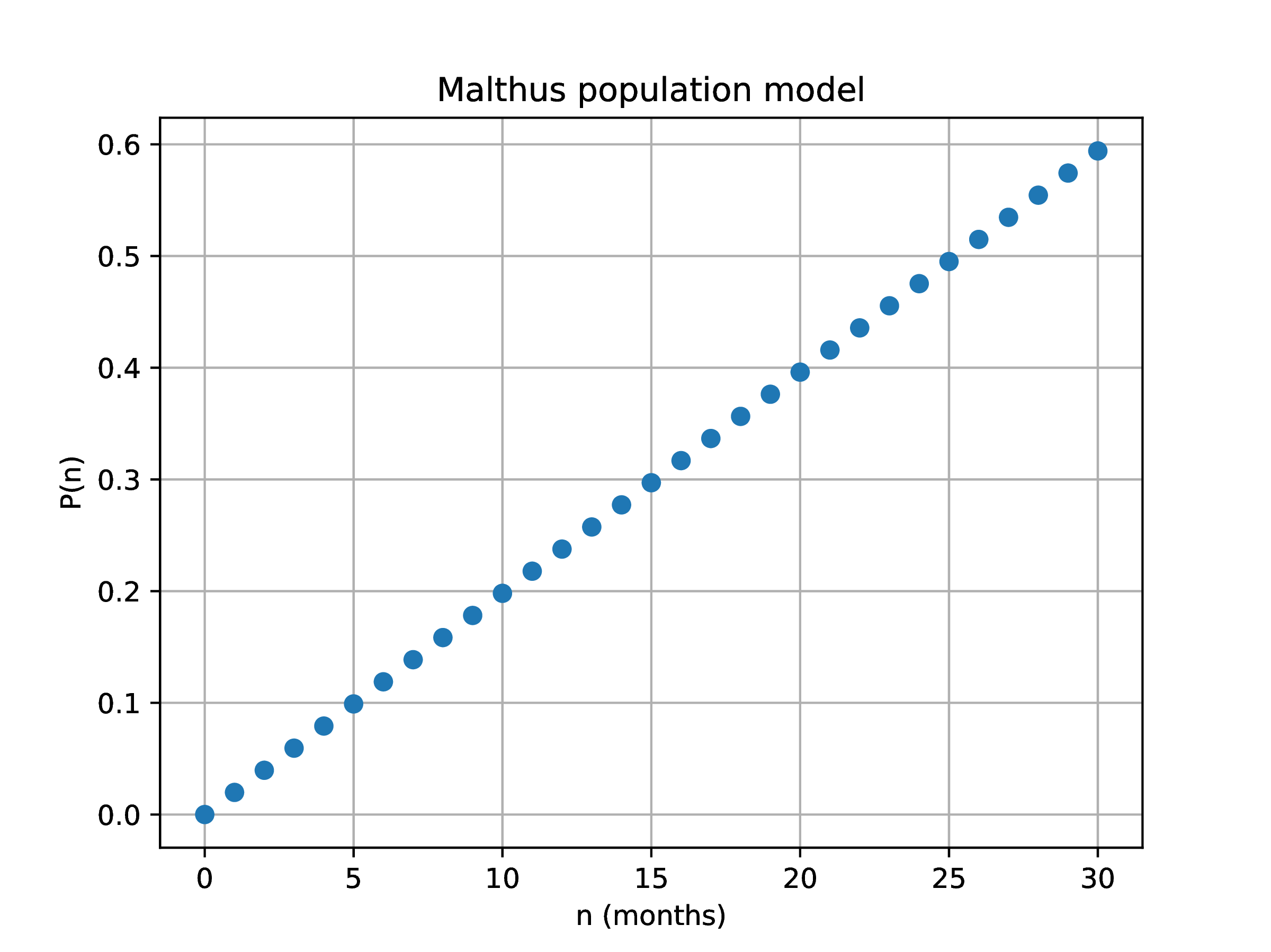
1.3Malthus population model

A different population model is given

∴ 

function P(n,r)
  if ((typeof(n)==Int64) && (n>=0) && (r>-1))
    if (n==0) 
       return 1
    end
    return (1+r)*P(n-1,r)
  else
    print("Invalid argument\n")
  end
end

∴ 

P(2,0.1)

∴ 

$•$

Figure 2.

∴	N=30; n=0:N; r=1; Pn=P.(n,r); plot(n,log.(Pn),"o");

∴	xlabel("n (months)"); ylabel("P(n)");

∴	title("Malthus population model"); grid("on");

∴	savefig(homedir() * "/courses/MATH089/images/Malthus.eps")

∴

1.4Logistic population model

2Systems of difference equations

2.1Predator-prey models

2.1.1Hypotheses

2.1.2Mathematical model

2.1.3Implementation

∴ 

r=0.01; a=0.02; s=0.005; b=0.1; A=100; B=1000;

∴ 

function WS(n)
  global r,s,a,b,A,B
  if ((typeof(n)==Int64) && (n>=0))
    if (n==0)
      return [A B]
    else
      W = WS(n-1)[1] + r*WS(n-1)[1]*WS(n-1)[2] - a*WS(n-1)[1]
      S = WS(n-1)[2] - s*WS(n-1)[1]*WS(n-1)[2] + b*WS(n-1)[2]
      return [W S]
    end
  else
    print("Invalid argument")
  end
end

∴ 

WS(3)

∴ 

x[1]

∴ 

x[2]

∴ 

2.1.4Results and discussion

2.2Resource-Grazer-Predator models

2.3Susceptible-Infectious-Recovered disease propagation models