|
Posted: 11/1/21
Due: 11/12/21, 11:55PM
This project investigates models based upon random realizations of some process, an approach known as Monte Carlo simulation. After an introductory example on approximation of by random throws of a needle against a pattern of parallel lines (Buffon's needle), approaches to grouping connected entities to maximize some goal is considered. This is a generic problem arising in many fields such as allocation of economic resources or social network analysis. The example considered here is that of election district formation in North Carolina by grouping counties, an application relevant to the topical conversation of gerrymandering.
Tasks:
Buffon needle convergence plot
Monte Carlo districting
(In your own words, describe Monte Carlo simulation and gerrymandering. Make reference to the background paper presented in class)
(Describe the Buffon needle problem, define Julia functions to find the crossing probability, and provide a plot of the estimation of )
∴ |
function πBuffon(l,t,n) N=Int(trunc(n)) x=t*rand(N); θ=π*rand(N); c=cos.(θ) nlft = sum(x .- l*c .<= 0) nrgt = sum(x .+ l*c .>= t) p = (nlft+nrgt)/N return 2*l/t/p end |
πBuffon
∴ |
πBuffon(0.5,1,1.0e6) |
∴ |
πBuffon.(0.5,1,(5:5:20)*1.0e6)' |
(1)
∴ |
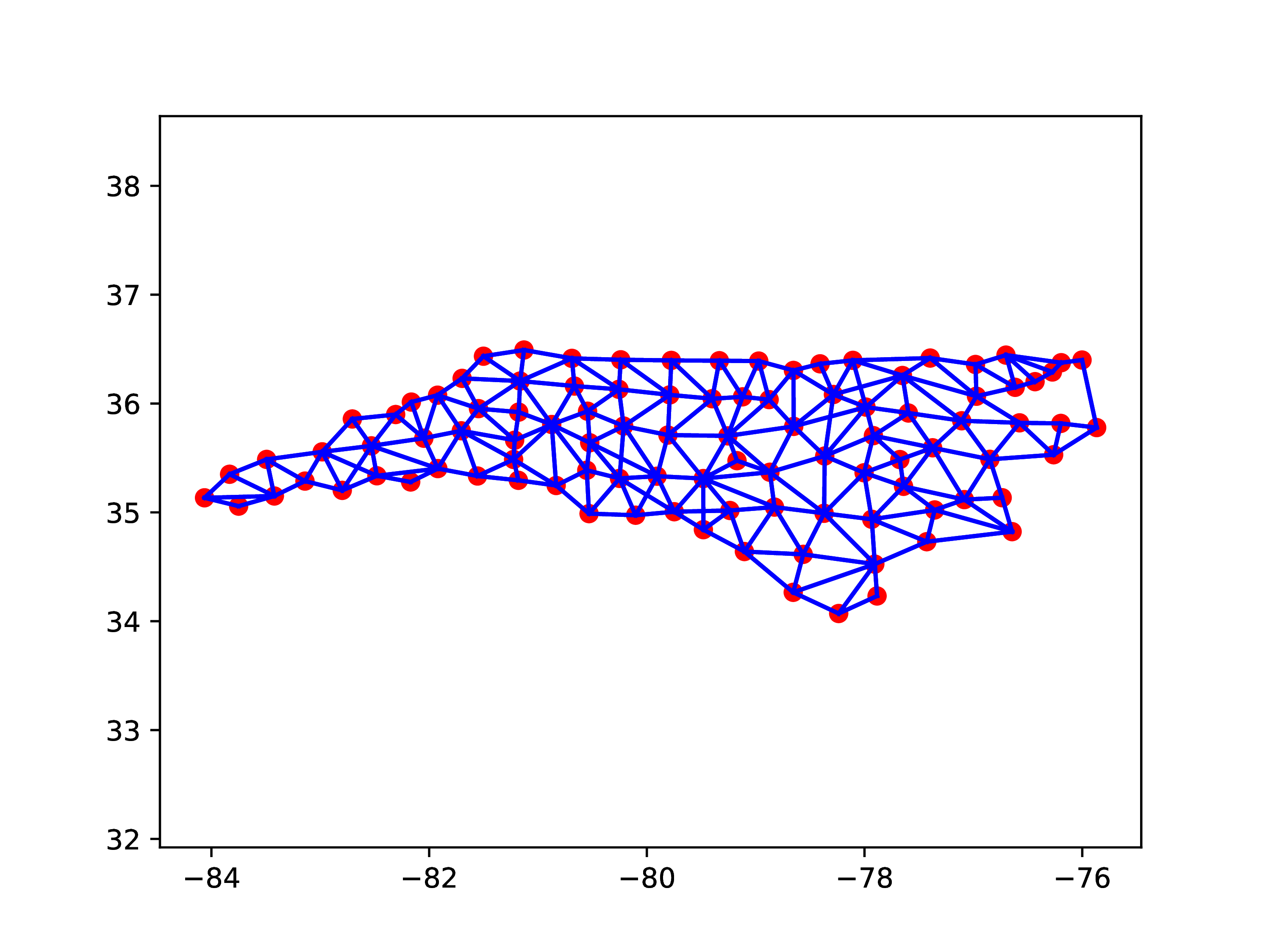
(A graph is a structure containing vertices and edges. Describe representation of NC counties by a graph)
This folded code adds a package to Julia that enables the reading of Matlab files. It only needs to be run once.
This folded code reads NC data
∴ |
using MAT |
∴ |
cd("/home/student/courses/MATH089/voting") |
∴ |
data=matread("NCcounties.mat")["Expression1"]; |
∴ |
nCounties, nData=size(data) |
(2)
∴ |
pop=data[:,1]; y=data[:,2]; x=data[:,3]; |
∴ |
nNeighbors=Int.(trunc.(data[:,4])); |
∴ |
Neighbors=Int.(trunc.(data[:,5:13])); |
∴ |
Grouping counties into electoral districts is a particular case of the general problem of placing objects into groups. Denote by the number of objects in group . The total number of choices for the first group is known as a combination and given by
Estimation of number of choices is aided by Stirling's formula
giving, for instance, the estimate
The total number of groupings of counties into districts is given by the sum
Extra credit: Find the number of possible groupings of North Carolina counties.
Decisions on whether one districting choice is better than another requires the definition of quantitative criteria that can be optimized. Many such criteria can be generated, but two simple choices are considered here.
The center of gravity of district is given by the first moments
where is the index of the county out of the counties in district .
How much a district is stretched in the coordinates is given by the centered second moments (variances)
The ratio is close to one for an approximately circular district, hence the function
is an overall descriptor of geographical skewness of districting .
Another possible criterion is equal populations in each district, given by the descriptor
with the population in district , and the desired population equal to overall population divided by number of counties.
In a Monte Carlo approach, random choices of groupings are attempted, and a record is kept of the grouping that optimizes the goal function. Assume the goal function is
which should be as small as possible. The weight determines the relative importance of each criterion.
∴ |
function genD(m,n,v)
   nCD = Int(trunc(n/m)) # Average nr. of counties per district
   D = fill(0,m,2*nCD)   # Allocate space: counties in each district
   nD = fill(0,m)        # Allocate space: nr. of counties in district
   C = collect(1:n)      # List of counties to be distributed
   nC = n                # Nr. of counties that can be distributed
   for i=1:m-1           # Loop over districts
     # Nr. of counties to be placed in district i
     nDi = rand(nCD-v:nCD+v) # Random number close to average
     nDi = min(nDi,nC)   # Cannot be more than available counties
     nDi = max(1,nDi)    # Has to be at least one county
     nD[i] = nDi         # Store number of counties in district
     for k=1:nD[i]       # Loop over nr. of counties to be placed in i
        ic = rand(1:nC)  # Generate a random number to choose county
        D[i,k] = C[ic]   # Place county C[ic] in district i at pos. k
        C[ic:nC-1] = C[ic+1:nC] # Erase county from available counties
        nC = nC - 1      # One less county to distribute
        #@printf("i=%d k=%d ic=%d nC=%d\n",i,k,ic,nC)
        if (nC==0)       # Stop if there are no more counties
          break
        end
     end
     if (nC==0) break; end
   end
   # Last district contains remaining counties
   if (nC>0)
     nD[m] = nC; D[m,1:nC]=C[1:nC]
   end
   return nD,D
end; |
∴ |
nD,D=genD(13,100,3) |
(3)
∴ |
sum(nD) |
∴ |
D |
(4)
∴ |
(Present a log-log plot of the error in estimation of in the Buffon needle with respect to the number of throws. Estimate te slope of the log-log plot).
(Present a plot of the values of the goal function for many districting attempts. Present a table of the five best districting choices. Attempt to plot the best districting you've found)
(Present your conclusions on the use of random numbers to simulate real-life models)