MATH347

MATH347 L20: Least squares applications

Recall: least squares problem formulation/solution

Consider approximating $𝒃 \in ℝ^{m}$ by linear combination of $n$ vectors, $𝑨 \in ℝ^{m \times n}$
Make approximation error $𝒆 = 𝒃 - 𝒗 = 𝒃 - 𝑨 𝒙$ as small as possible
${min}_{𝒙 \in ℝ^{n}} {|| 𝒃 - 𝑨 𝒙 ||}_{2}$
Error is measured in the 2-norm $\Rightarrow$ the least squares problem (LSQ)
Solution is the projection of $𝒃$ onto $C (𝑨)$
$𝑸 𝑹 = 𝑨, 𝑷_{C (𝑨)} = 𝑸 𝑸^{T}, 𝒗 = (𝑸 𝑸^{T}) 𝒃$
The vector $𝒙$ is found by back-substitution from
$𝒗 = (𝑸 𝑸^{T}) 𝒃 = (𝑸 𝑹) 𝒙 \Rightarrow 𝑹 𝒙 = 𝑸^{T} 𝒃 .$

Applications: polynomial approximations

LSQ has myriad applications throughout science
Consider data $𝒟 = {(x_{i}, y_{i}), i = 1, \dots, m}$
The polynomial interpolant of degree $m - 1$ passes through the data points
$p_{m - 1} (x) = c_{0} + c_{1} x + \dots + c_{m - 1} x^{m - 1} = [\begin{array}{llll} 1 & x & \dots & x^{m - 1} \end{array}] 𝒄$
Impose conditions $p_{m - 1} (x_{i}) = y_{i}, i = 1, \dots, m$ to obtain linear system
$[\begin{array}{lllll} 1 & x_{1} & x_{1}^{2} & \dots & x_{1}^{m - 1} \\ 1 & x_{2} & x_{2}^{2} & \dots & x_{2}^{m - 1} \\ ⋮ & ⋮ & ⋮ & ⋱ & ⋮ \\ 1 & x_{m} & x_{m}^{2} & \dots & x_{m}^{m - 1} \end{array}] [\begin{array}{l} c_{0} \\ c_{1} \\ c_{2} \\ ⋮ \\ c_{m - 1} \end{array}] = [\begin{array}{l} y_{1} \\ y_{2} \\ y_{3} \\ ⋮ \\ y_{m} \end{array}] \Rightarrow 𝑨 𝒄 = 𝒚, 𝑨 \in ℝ^{m \times m}$
>>

m=4; x=transpose(1:m); y=1 - 2*x + 3*x.^2 - 4*x.^3;
>>

A=[x.^0 x.^1 x.^2 x.^3]; [Q,R]=qr(A); c = R \ (Q'*y); c'
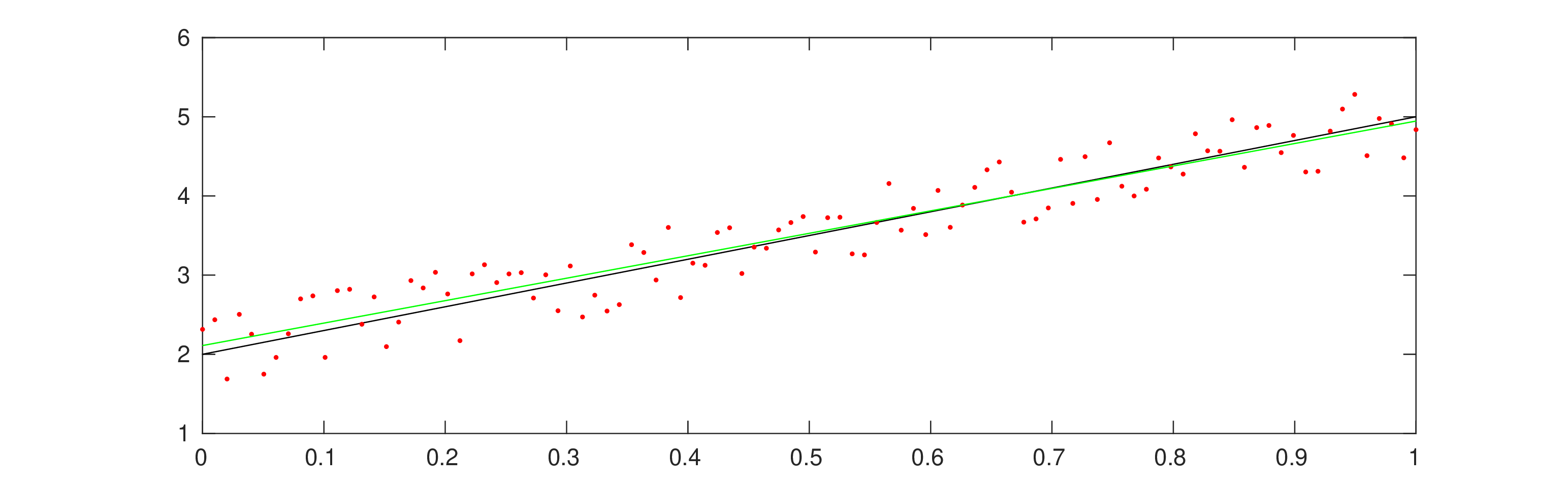
$(\begin{array}{cccc} 1.0000 & - 2.0000 & 3.0000 & - 4.0000 \end{array})$

LSQ polynomial approximant - first degree (linear regression)

Consider noisy data containing many measurements $𝒟 = {(x_{i}, y_{i}), i = 1, \dots, m}$

Assume data without noise would conform to some polynomial law

y_{i} = z_{i} + r_{i} = c_{0} + c_{1} x_{i} + r_{i}, i = 1, \dots, m

with $r_{i}$ a random number uniformly distributed within $(- R, R)$ .

>>	m=100; x=linspace(0,1,m)';

>>	c0=2; c1=3; z=c0+c1*x; y=(z+rand(m,1)-0.5);

>>	A=ones(m,2); A(:,2)=x(:); [Q,R]=qr(A); c = R \ (Q'*y); c'

$(\begin{array}{cc} 1.9506 & 3.0310 \end{array})$

>>	w=A*c; plot(x,z,'k',x,y,'.r',x,w,'g');

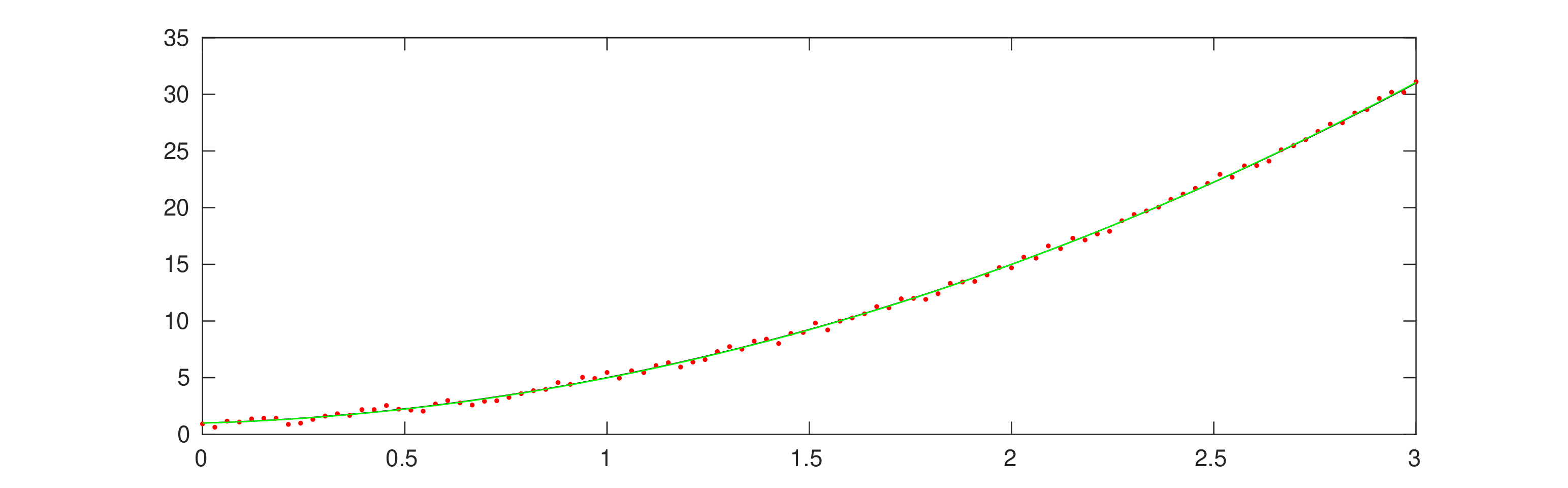
LSQ polynomial approximant - second degree

Consider noisy data containing many measurements $𝒟 = {(x_{i}, y_{i}), i = 1, \dots, m}$

Assume data without noise would conform to some polynomial law

y_{i} = z_{i} + r_{i} = c_{0} + c_{1} x_{i} + r_{i}, i = 1, \dots, m

with $r_{i}$ a random number uniformly distributed within $(- R, R)$ .

>>	m=100; x=linspace(0,3,m)';

>>	c0=1; c1=1; c2=3; z=c0+c1x+c2x.^2; y=(z+rand(m,1)-0.5);

>>	A=ones(m,3); A(:,2)=x(:); A(:,3)=x(:).^2; [Q,R]=qr(A); c=R\(Q'*y); c'

$(\begin{array}{ccc} 1.0047 & 0.9641 & 3.0143 \end{array})$

>>	w=A*c; plot(x,z,'k',x,y,'.r',x,w,'g');