MATH347 L24: SVD computation and applications

• New concepts:

  • SVD computation

  • Matrix norm

  • Low-rank approximations

  • Image compression

SVD diagram

• SVD of \(\boldsymbol{A} \in \mathbb{R}^{m \times n}\) reveals: \(\operatorname{rank} (\boldsymbol{A})\), bases for \({\color{blue}{{C (\boldsymbol{A})}}}, {\color{red}{N (\boldsymbol{A}^T)}}, {\color{blue}{C (\boldsymbol{A}^T)}}, {N (\boldsymbol{A})}\)

SVD Computation

• From \(\boldsymbol{A}=\boldsymbol{U}\boldsymbol{\Sigma}\boldsymbol{V}^T\) deduce \(\boldsymbol{A}\boldsymbol{A}^T =\boldsymbol{U}\boldsymbol{\Sigma}^2 \boldsymbol{U}^T\), \(\boldsymbol{A}^T \boldsymbol{A}=\boldsymbol{V}\boldsymbol{\Sigma}^2 \boldsymbol{V}^T\), hence \(\boldsymbol{U}\) is the eigenvector matrix of \(\boldsymbol{A}\boldsymbol{A}^T\), and \(\boldsymbol{V}\) is the eigenvector matrix of \(\boldsymbol{A}^T \boldsymbol{A}\)

• SVD computation is carried out by solving eigenvalue problems

  matlab>>

  A=[2 -1; -3 1]; [U S2]=eig(A*A'); [V S2]=eig(A'*A); S=sqrt(S2); disp([ U S V']);

  >> -0.8174 -0.5760 0.2588 0 -0.3606 -0.9327

  -0.5760 0.8174 0 3.8643 -0.9327 0.3606

  The above is not an SVD since the singular values on the diagonal are out of order. The matlab svd function returns the correct ordering.

  matlab>>

  [U S V]=svd(A); disp([U S V']);

  >> -0.5760 0.8174 3.8643 0 -0.9327 0.3606

  0.8174 0.5760 0 0.2588 -0.3606 -0.9327

• Hand computation of the SVD is a direct application of eigenvalue computation. Note that eigenvalues of \(\boldsymbol{A}\boldsymbol{A}^T\) and \(\boldsymbol{A}^T \boldsymbol{A}\) are identical, but the eigenvectors differ.

Matrix norm - a diagram for \(m = 2\)

• Construct a diagram of the SVD of \(\boldsymbol{A}= \left[ \begin{array}{ll} 2 & - 1\\ 3 & 1 \end{array} \right]\), with \(\boldsymbol{f} (\boldsymbol{x}) =\boldsymbol{A}\boldsymbol{x}\) the associated linear mapping by taking \(\theta \in [0, 2 \pi]\) and

  \(\displaystyle \boldsymbol{x}= \left[ \begin{array}{l} \cos \theta\\ \sin \theta \end{array} \right], \| \boldsymbol{x} \|_2 = 1\)

  traversing the unit circle in the domain of \(\boldsymbol{f}: \mathbb{R}^2 \rightarrow \mathbb{R}^2\). The image of the unit circle is an ellipse. The length of the semiaxes are the singular values of \(\boldsymbol{A}\), the orientation of the semiaxes are given by the right singular vectors \(\boldsymbol{U}\).

  

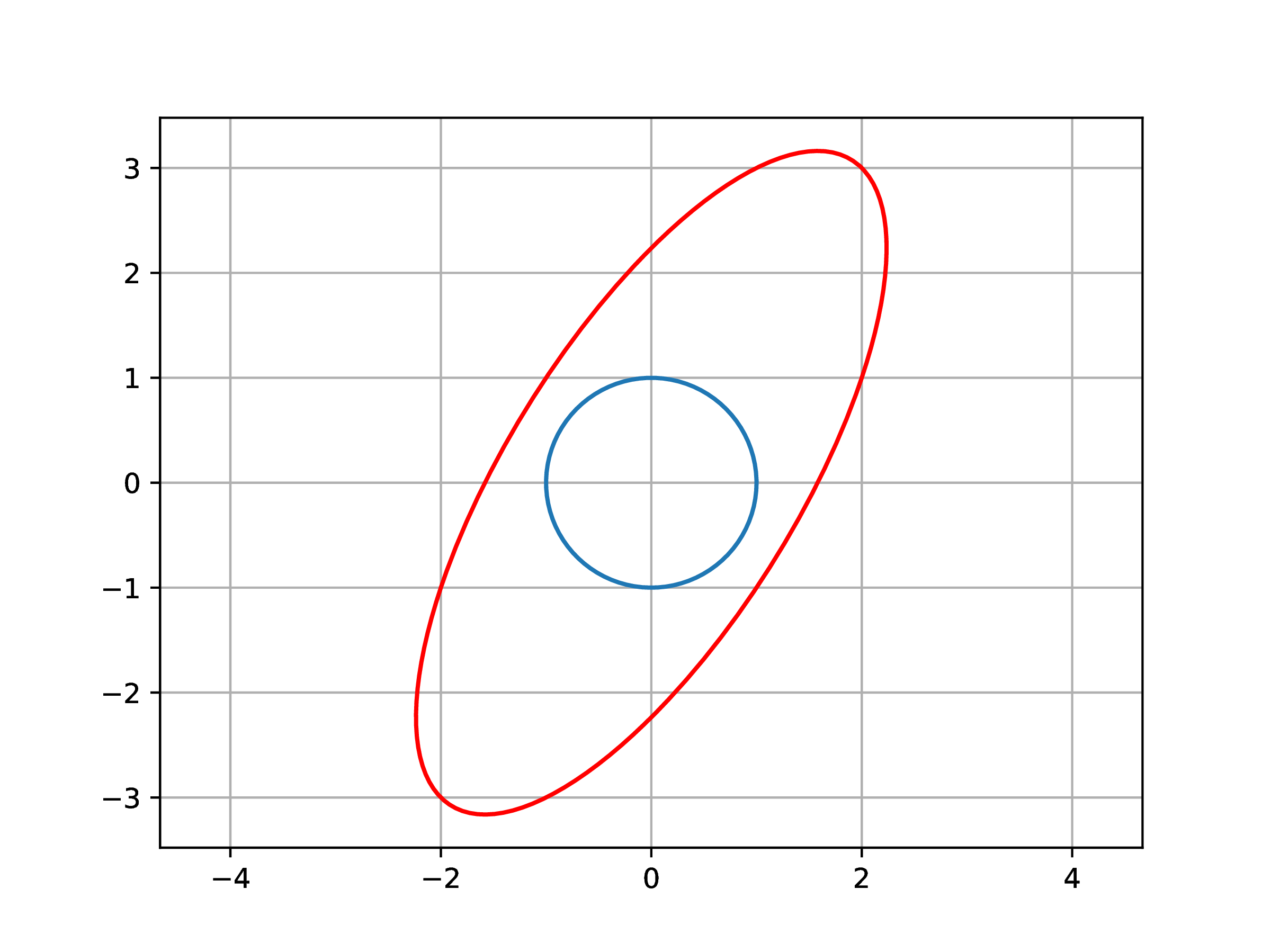
• The above offers a way to think about the “size” of a matrix as defined by the maximal amplification factor among all directions with the domain

Induced matrix norm

Definition. Given the vector norms \(\| \|_{(n)} : \mathbb{R}^n \rightarrow \mathbb{R}_+\). \(\| \|_{(m)} : \mathbb{R}^m \rightarrow \mathbb{R}_+\) for vector spaces \((\mathbb{R}^m, \mathbb{R}, +, \cdot)\), \((\mathbb{R}^n, \mathbb{R}, +, \cdot)\), the induced matrix norm of \(\boldsymbol{A} \in \mathbb{R}^{m \times n}\) is defined as

The above definition states that the “size” of a matrix can be interpreted as the maximal amplication factor among all possible orientations of a unit vector input.

• The most commonly encountered case is for both the \(\| \|_{(m)}\) and the \(\| \|_{(n)}\) norms to be 2-norms

  \(\displaystyle \| \boldsymbol{b} \|_{(m)} = \left( \sum_{i = 1}^m b_i^2 \right)^{1 / 2}, \| \boldsymbol{x} \|_{(n)} = \left( \sum_{i = 1}^n x_i^2 \right)^{1 / 2}\)

• When the vector norms are both 2-norms as above, the induced matrix norm is simply the largest singular value of \(\boldsymbol{A}\)

  \(\displaystyle \| \boldsymbol{A} \| = \sigma_1\)

Low-rank matrix approximation

• Full SVD

  \(\displaystyle \boldsymbol{A}= \sum_{i = 1}^r \sigma_i \boldsymbol{u}_i \boldsymbol{v}_i^T, r \leqslant \min (m, n) .\)

• Truncated SVD

  \(\displaystyle \boldsymbol{A} \cong \boldsymbol{A}_p = \sum_{i = 1}^p \sigma_i \boldsymbol{u}_i \boldsymbol{v}_i^T .\)

  Interpret \(\boldsymbol{A}_p\) as furnishing an approximation to \(\boldsymbol{A}\), with \(\operatorname{rank} (\boldsymbol{A}_p) = p \leqslant r\).

• Many applications, e.g., image compression