MATH347 Course review

• What is linear algebra and why is to so important to so many applications?

• Basic operations: defined to express linear combination

• Linear operators, Fundamental Theorem of Linear Algebra (FTLA)

• Factorizations: more convenient expression of linear combination

  \(\displaystyle \boldsymbol{L}\boldsymbol{U}=\boldsymbol{A}, \boldsymbol{Q}\boldsymbol{R}=\boldsymbol{A}, \boldsymbol{X}\boldsymbol{\Lambda}\boldsymbol{X}^{- 1} =\boldsymbol{A}, \boldsymbol{U}\boldsymbol{\Sigma}\boldsymbol{V}^T =\boldsymbol{A}\)

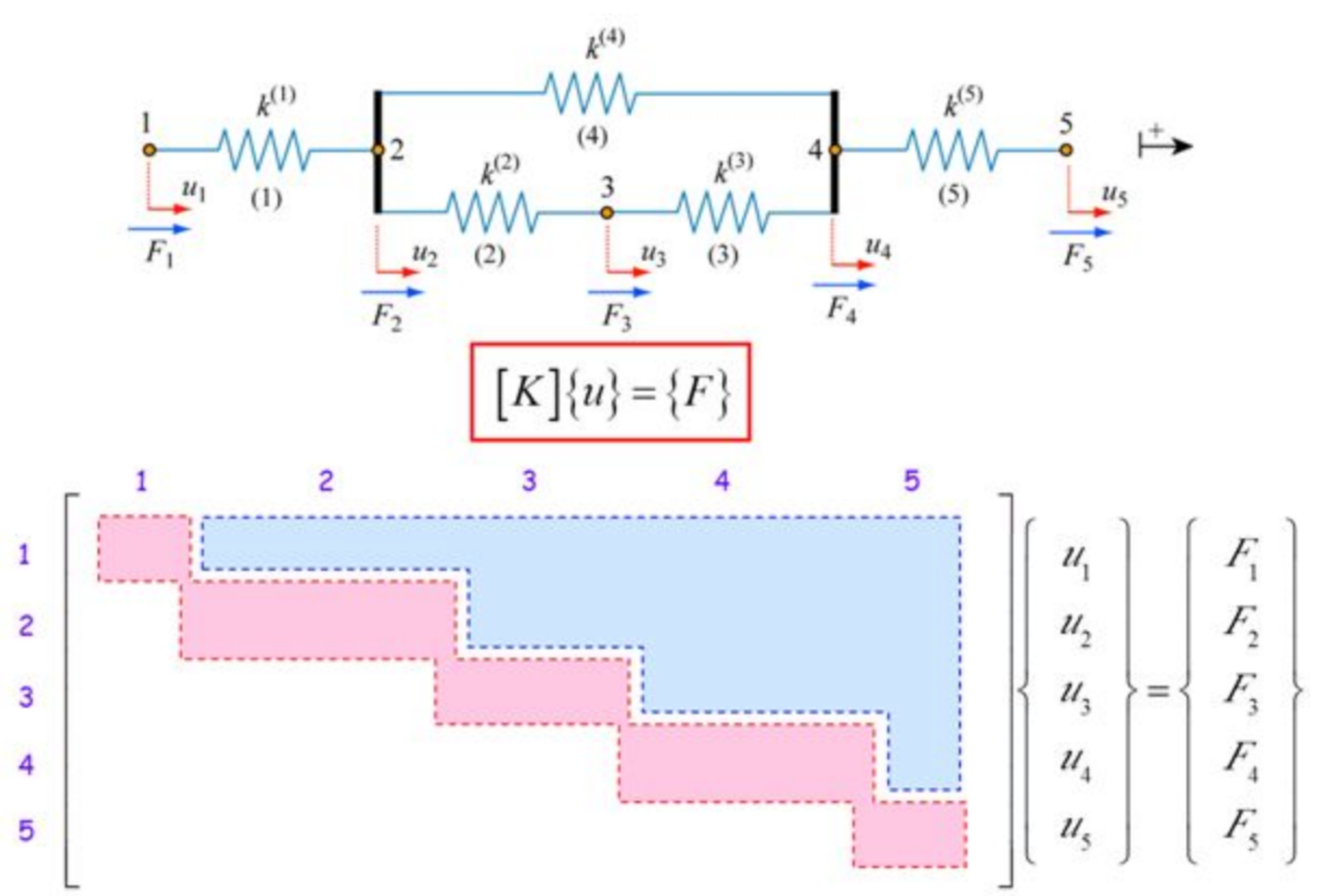
• Solving linear systems (change of basis) \(\boldsymbol{I}\boldsymbol{b}=\boldsymbol{A}\boldsymbol{x}\)

• Best 2-norm approximation: least squares \(\min_{\boldsymbol{x}} \| \boldsymbol{b}-\boldsymbol{A}\boldsymbol{x} \|_2\)

• Exposing the structure of a linear operator between the same sets through eigendecomposition

• Exposing the structure of a linear operator between different sets through the SVD

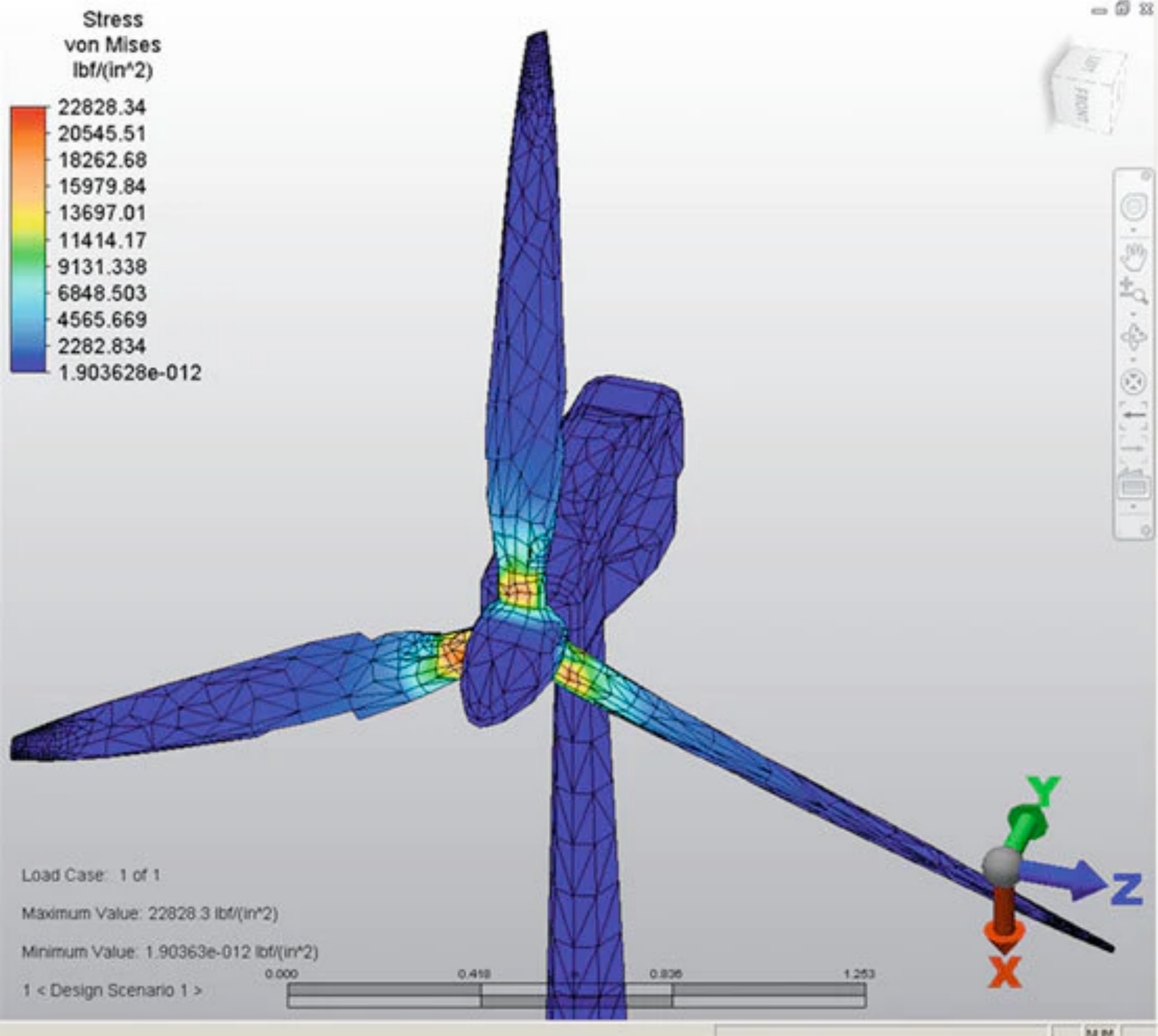
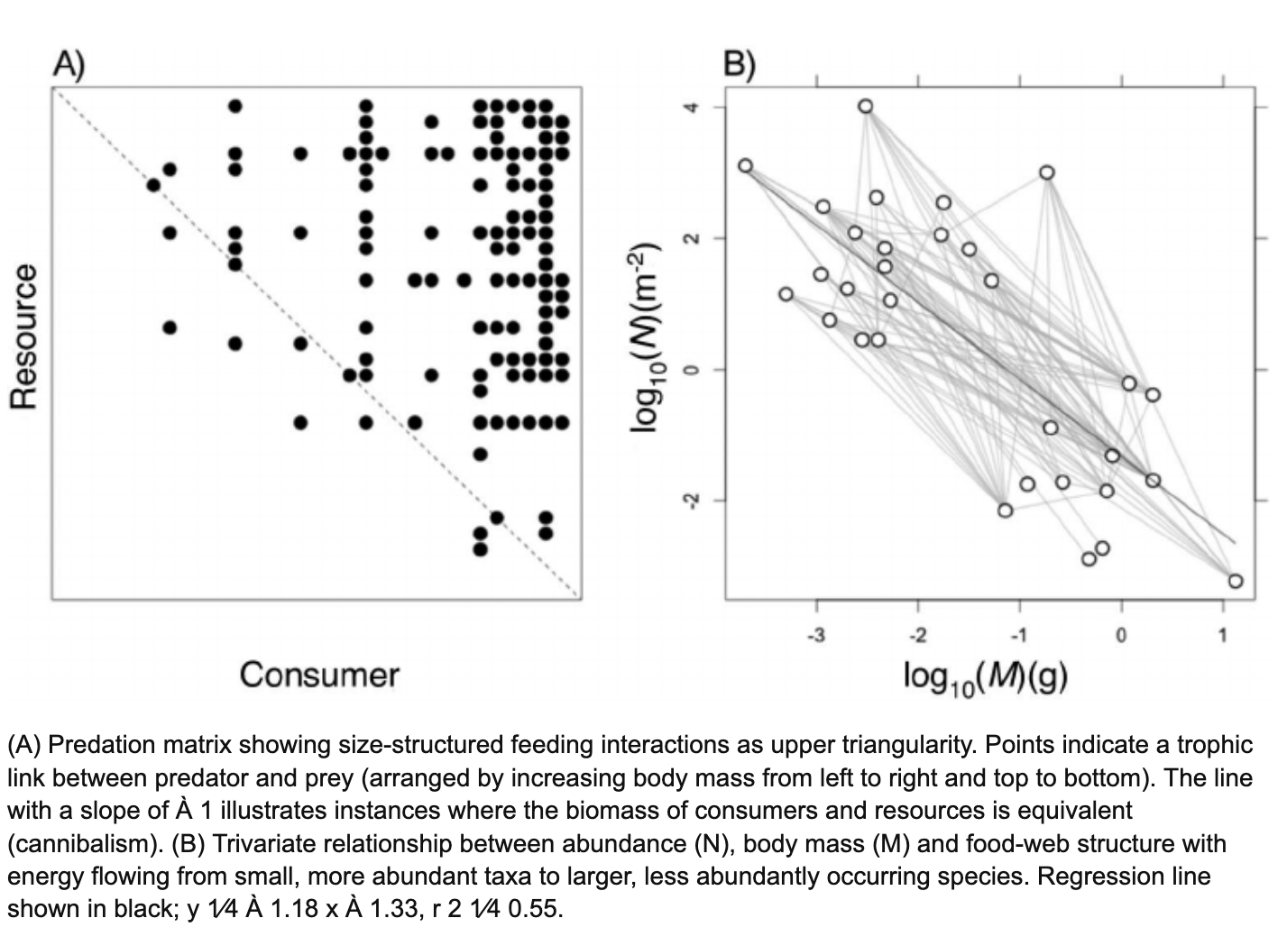
• Applications: any type of correlation

What is linear algebra, and why is it important?

• Science acquires and organizes knowledge into theories that can be verified by quantified tests. Mathematics furnishes the appropriate context through rigorous definition of \(\mathbb{N}, \mathbb{R}, \mathbb{Q}, \mathbb{C}\).

• Most areas of science require groups of numbers to describe an observation. To organize knowledge rules on how such groups of numbers may be combined are needed. Mathematics furnishes the concept of a vector space \((\mathcal{S}, \mathcal{V}, +)\)

  1. formal definition of a single number: scalar, \(\alpha, \beta \in \mathcal{S}\)

  2. formal definition of a group of numbers: vector, \(\boldsymbol{u}, \boldsymbol{v} \in \mathcal{V}\)

  3. formal definition of a possible way to combine vectors: \(\alpha \boldsymbol{u}+ \beta \boldsymbol{v}\)

• Algebra is concerned with precise definition of ways to combine mathematical objects, i.e., to organize more complex knowledge as a sequence of operations on simpler objects

• Linear algebra concentrates on one particular operation: the linear combination \(\alpha \boldsymbol{u}+ \beta \boldsymbol{v}\)

• It turns out that a complete theory can be built around the linear combination, and this leads to the many applications linear algebra finds in all branches of knowledge.

Basic operations, concepts

• Group vectors as column vectors into matrices \(\boldsymbol{A}= \left( \begin{array}{llll} \boldsymbol{a}_1 & \boldsymbol{a}_2 & \ldots & \boldsymbol{a}_n \end{array} \right) \in \mathbb{R}^{m \times n}\)

• Define matrix-vector multiplication to express the basic linear combination operation

  \(\displaystyle \boldsymbol{b}=\boldsymbol{A}\boldsymbol{x}= x_1 \boldsymbol{a}_1 + \ldots + x_n \boldsymbol{a}_n\)

• Introduce a way to switch between column and row storage through the transposition operation \(\boldsymbol{A}^T\). \((\boldsymbol{A}+\boldsymbol{B})^T =\boldsymbol{A}^T +\boldsymbol{B}^T\), \((\boldsymbol{A}\boldsymbol{B})^T =\boldsymbol{B}^T \boldsymbol{A}^T\)

• Transform between one set of basis vectors and another \(\boldsymbol{b}\boldsymbol{I}=\boldsymbol{A}\boldsymbol{x}\)

• Linear independence establishes when a vector cannot be described as a linear combination of other vectors, i.e., if the only way to satisfy \(x_1 \boldsymbol{a}_1 + \ldots + x_n \boldsymbol{a}_n =\boldsymbol{0}\) is for \(x_1 = \ldots = x_n = 0\), then the vectors \(\boldsymbol{a}_1, \ldots, \boldsymbol{a}_n\) are linearly independent

• The span \(\langle \boldsymbol{a}_1, \ldots, \boldsymbol{a}_n \rangle = \{ \boldsymbol{b} | \exists \boldsymbol{x} \in \mathbb{R}^n \operatorname{such}\operatorname{that}\boldsymbol{b}= x_1 \boldsymbol{a}_1 + \ldots x_n \boldsymbol{a}_n \}\) is the set of all vectors is reachable by linear combination of \(\boldsymbol{a}_1, \ldots, \boldsymbol{a}_n\)

• The set of vectors \(\{ \boldsymbol{a}_1, \ldots, \boldsymbol{a}_n \}\) is a basis of a vector space \(\mathcal{V}\) if \(\langle \boldsymbol{a}_1, \ldots, \boldsymbol{a}_n \rangle =\mathcal{V}\), and \(\boldsymbol{a}_1, \ldots, \boldsymbol{a}_n\) are linearly independent

• The number of vectors in a basis is the dimension of a vector space.

Characterization of a linear operator

• Any linear operator \(T : \mathcal{D} \rightarrow \mathcal{C}\), \(T (\alpha \boldsymbol{u}+ \beta \boldsymbol{v}) = \alpha T (\boldsymbol{u}) + \beta T (\boldsymbol{v})\) can be characterized by a matrix \(\boldsymbol{A}= \left[ \begin{array}{llll} T (\boldsymbol{e}_1) & T (\boldsymbol{e}_2) & \ldots & T (\boldsymbol{e}_n) \end{array} \right]\)

• For each matrix \(\boldsymbol{A} \in \mathbb{R}^{m \times n}\) there exist four fundamental subspaces:

  1. Column space, \(C (\boldsymbol{A}) = \{ \boldsymbol{b} \in \mathbb{R}^m | \exists \boldsymbol{x} \in \mathbb{R}^n \operatorname{such}\operatorname{that}\boldsymbol{b}=\boldsymbol{A}\boldsymbol{x} \} \subseteq \mathbb{R}^m\), the part of \(\mathbb{R}^m\) reachable by linear combination of columns of \(\boldsymbol{A}\)

  2. Left null space, \(N (\boldsymbol{A}^T) = \{ \boldsymbol{y} \in \mathbb{R}^m | \boldsymbol{A}^T \boldsymbol{y}= 0 \} \subseteq \mathbb{R}^m\), the part of \(\mathbb{R}^m\) not reachable by linear combination of columns of \(\boldsymbol{A}\)

  3. Row space, \(R (\boldsymbol{A}) = C (\boldsymbol{A}^T) = \{ \boldsymbol{c} \in \mathbb{R}^n | \exists \boldsymbol{y} \in \mathbb{R}^m \operatorname{such}\operatorname{that}\boldsymbol{c}=\boldsymbol{A}^T \boldsymbol{y} \} \subseteq \mathbb{R}^n\), the part of \(\mathbb{R}^m\) reachable by linear combination of rows of \(\boldsymbol{A}\)

  4. Null space, \(N (\boldsymbol{A}) = \{ \boldsymbol{x} \in \mathbb{R}^n | \boldsymbol{A}\boldsymbol{x}= 0 \} \subseteq \mathbb{R}^n\), the part of \(\mathbb{R}^m\) not reachable by linear combination of rows of \(\boldsymbol{A}\)

  The fundamental theorem of linear algebra (FTLA) states

  \begin{eqnarray*} C (\boldsymbol{A}), N (\boldsymbol{A}^T) \leq \mathbb{R}^m, C (\boldsymbol{A}) \bot N (\boldsymbol{A}^T), & C (\boldsymbol{A}) \cap N (\boldsymbol{A}^T) = \{ \boldsymbol{0} \}, & C (\boldsymbol{A}) \oplus N (\boldsymbol{A}^T) =\mathbb{R}^m\\ C (\boldsymbol{A}^T), N (\boldsymbol{A}) \leq \mathbb{R}^n, C (\boldsymbol{A}^T) \bot N (\boldsymbol{A}), & C (\boldsymbol{A}^T) \cap N (\boldsymbol{A}) = \{ \boldsymbol{0} \}, & C (\boldsymbol{A}^T) \oplus N (\boldsymbol{A}) =\mathbb{R}^n \end{eqnarray*}

Factorizations

• \(\boldsymbol{L}\boldsymbol{U}=\boldsymbol{A}\), (or \(\boldsymbol{L}\boldsymbol{U}=\boldsymbol{P}\boldsymbol{A}\) with \(\boldsymbol{P}\) a permutation matrix) Gaussian elimination, solving linear systems. Given \(\boldsymbol{A} \in \mathbb{R}^{m \times m}, \boldsymbol{b} \in \mathbb{R}^m\), \(\boldsymbol{b} \in C (\boldsymbol{A})\), find \(\boldsymbol{x} \in \mathbb{R}^m\) such that \(\boldsymbol{A}\boldsymbol{x}=\boldsymbol{b}=\boldsymbol{I}\boldsymbol{b}\) by:

  1. Factorize, \(\boldsymbol{L}\boldsymbol{U}=\boldsymbol{P}\boldsymbol{A}\)

  2. Solve lower triangular system \(\boldsymbol{L}\boldsymbol{y}=\boldsymbol{P}\boldsymbol{b}\) by forward substitution

  3. Solve upper triangular system \(\boldsymbol{U}\boldsymbol{x}=\boldsymbol{y}\) by backward substitution

• \(\boldsymbol{Q}\boldsymbol{R}=\boldsymbol{A}\), (or \(\boldsymbol{Q}\boldsymbol{R}=\boldsymbol{P}\boldsymbol{A}\) with \(\boldsymbol{P}\) a permutation matrix) Gram-Schmidt, solving least squares problem. Given \(\boldsymbol{A} \in \mathbb{R}^{m \times n}\), \(\boldsymbol{b} \in \mathbb{R}^m\), \(n \leqslant m\), solve \(\min_{\boldsymbol{x} \in \mathbb{R}^n} \| \boldsymbol{b}-\boldsymbol{A}\boldsymbol{x} \|\) by:

  1. Factorize, \(\boldsymbol{Q}\boldsymbol{R}=\boldsymbol{P}\boldsymbol{A}\)

  2. Solve upper triangular system \(\boldsymbol{R}\boldsymbol{x}=\boldsymbol{Q}^T \boldsymbol{b}\) by forward substitution

  \(\boldsymbol{X}\boldsymbol{\Lambda}\boldsymbol{X}^{- 1} =\boldsymbol{A}\), eigendecomposition of \(\boldsymbol{A} \in \mathbb{R}^{m \times m}\) (\(\boldsymbol{X}\) invertible if \(\boldsymbol{A}\) is normal, i.e., \(\boldsymbol{A}\boldsymbol{A}^T =\boldsymbol{A}^T \boldsymbol{A}\))

• \(\boldsymbol{Q}\boldsymbol{\Lambda}\boldsymbol{Q}^T =\boldsymbol{A}\), orthogonal eigendecomposition when \(\boldsymbol{A}\boldsymbol{A}^T =\boldsymbol{A}^T \boldsymbol{A}\) (normal)

• \(\boldsymbol{Q}\boldsymbol{T}\boldsymbol{Q}^T =\boldsymbol{A}\), Schur decomposition of \(\boldsymbol{A} \in \mathbb{R}^{m \times m}\), \(\boldsymbol{Q}\) orthogonal matrix, \(\boldsymbol{T}\) triangular matrix, decomposition always exists

• \(\boldsymbol{U}\boldsymbol{\Sigma}\boldsymbol{V}^T =\boldsymbol{A}\), Singular value decomposition of \(\boldsymbol{A} \in \mathbb{R}^{m \times n}\), \(\boldsymbol{U} \in \mathbb{R}^{m \times m}, \boldsymbol{V} \in \mathbb{R}^{n \times n}\) orthogonal matrices, \(\boldsymbol{\Sigma}=\operatorname{diag} (\sigma_1, \sigma_2, \ldots) \in \mathbb{R}_+^{m \times n}\), decomposition always exists

Solving \(\boldsymbol{A}\boldsymbol{x}=\boldsymbol{b}\) by Gaussian elimination

• Gaussian elimination produces a sequence matrices similar to \(\boldsymbol{A} \in \mathbb{R}^{m \times m}\)

  \(\displaystyle \boldsymbol{A}=\boldsymbol{A}^{(0)} \sim \boldsymbol{A}^{(1)} \sim \cdots \sim \boldsymbol{A}^{(k)} \sim \cdots \sim \boldsymbol{A}^{(m - 1)}\)

• Step \(k\) produces zeros underneath diagonal position \((k, k)\)

• Step \(k\) can be represented as multiplication by matrix

  \(\displaystyle \boldsymbol{A}^{(k)} =\boldsymbol{L}_{_k} \boldsymbol{A}^{(k - 1)}, \boldsymbol{L}_k = \left( \begin{array}{ccccc} 1 & \ldots & 0 & \ldots & 1\\ 0 & \ddots & 0 & \ldots & 0\\ 0 & \ldots & 1 & \ldots & 0\\ 0 & \ldots & - l_{k + 1, k} & \ldots & 0\\ \vdots & \ldots & \vdots & \ddots & \vdots\\ 0 & \ldots & - l_{m, k} & \ldots & 1 \end{array} \right), l_{j, k} = \frac{{a_{j, k}^{(k - 1)}} }{a_{k, k}^{(k - 1)}}, \boldsymbol{A}^{(k)} = [a^{(k)}_{i, j}]\)

• All \(m - 1\) steps produce an upper triangular matrix

  \(\displaystyle \boldsymbol{L}_{m - 1} \ldots \boldsymbol{L}_2 \boldsymbol{L}_1 \boldsymbol{A}=\boldsymbol{U} \Rightarrow \boldsymbol{A}=\boldsymbol{L}_1^{- 1} \boldsymbol{L}_2^{- 1} \ldots \boldsymbol{L}_{m - 1}^{- 1} \boldsymbol{U}=\boldsymbol{L}\boldsymbol{U}\)

• With permutations \(\boldsymbol{P}\boldsymbol{A}= \boldsymbol{L}\boldsymbol{U}\) (Matlab [L,U,P]=lu(A), A=P'*L*U)

Matrix formulation of Gaussian elimination

• With known \(L U\)-factorization: \(\boldsymbol{A}\boldsymbol{x}=\boldsymbol{b} \Rightarrow (\boldsymbol{L}\boldsymbol{U}) \boldsymbol{x}=\boldsymbol{P}\boldsymbol{b} \Rightarrow \boldsymbol{L} (\boldsymbol{U}\boldsymbol{x}) =\boldsymbol{P}\boldsymbol{b}\)

• To solve \(\boldsymbol{A}\boldsymbol{x}=\boldsymbol{b}\):

  1. Carry out \(L U\)-factorization: \(\boldsymbol{P}^T \boldsymbol{L}\boldsymbol{U}=\boldsymbol{A}\)

  2. Solve \(\boldsymbol{L}\boldsymbol{y}=\boldsymbol{c}=\boldsymbol{P}\boldsymbol{b}\) by forward substitution to find \(\boldsymbol{y}\)

  3. Solve \(\boldsymbol{U}\boldsymbol{x}=\boldsymbol{y}\) by backward substitution

• FLOP = floating point operation = one multiplication and one addition

• Operation counts: how many FLOPS in each step?

  1. Each \(\boldsymbol{L}_k \boldsymbol{A}^{(k - 1)}\) costs \((m - k)^2\) FLOPS. Overall

     \(\displaystyle (m - 1)^2 + (m - 2)^2 + \cdots + 1^2 = \frac{m (m - 1) (2 m - 1)}{6} \approx \frac{m^3}{3}\)

  2. Forward substitution step \(k\) costs \(k\) flops

     \(\displaystyle 1 + 2 + \cdots + m = \frac{m (m + 1)}{2} \approx \frac{m^2}{2}\)

  3. Backward substitution cost is identical \(m (m + 1) / 2 \approx m^2 / 2\)/

Gram-Schmidt as \(\boldsymbol{Q}\boldsymbol{R}\)

• Orthonormalization of columns of \(\boldsymbol{A}\) is also a factorization

  \(\displaystyle \boldsymbol{A}= \left[ \begin{array}{llll} \boldsymbol{a}_1 & \boldsymbol{a}_2 & \ldots & \boldsymbol{a}_n \end{array} \right] = \left[ \begin{array}{llll} \boldsymbol{q}_1 & \boldsymbol{q}_2 & \ldots & \boldsymbol{q}_n \end{array} \right] \left[ \begin{array}{llll} r_{11} & r_{12} & \ldots & r_{1 n}\\ 0 & r_{22} & \ldots & r_{2 n}\\ \vdots & & \ddots & \\ 0 & 0 & \ldots & r_{n n} \end{array} \right] =\boldsymbol{Q}\boldsymbol{R}\) \(\displaystyle \begin{array}{l} \boldsymbol{a}_1 = r_{11} \boldsymbol{q}_1\\ \boldsymbol{a}_2 = r_{12} \boldsymbol{q}_1 + r_{2 2} \boldsymbol{q}_2\\ \boldsymbol{a}_3 = r_{13} \boldsymbol{q}_1 + r_{23} \boldsymbol{q}_2 + r_{3 3} \boldsymbol{q}_3\\ \vdots\\ \boldsymbol{a}_n = r_{1 n} \boldsymbol{q}_1 + r_{2 n} \boldsymbol{q}_2 + r_{3 n} \boldsymbol{q}_3 + \cdots + r_{n n} \boldsymbol{q}_n \end{array} \begin{array}{l} \boldsymbol{q}_1 =\boldsymbol{a}_1 / r_{11}\\ \boldsymbol{q}_2 = (\boldsymbol{a}_2 - r_{12} \boldsymbol{q}_1) / r_{2 2}\\ \boldsymbol{q}_3 = (\boldsymbol{a}_3 - r_{13} \boldsymbol{q}_1 - r_{23} \boldsymbol{q}_2) / r_{3 3}\\ \vdots \end{array}\)

• Operation count:

  • \(r_{j k} =\boldsymbol{q}_j^T \boldsymbol{a}_k\) costs \(m\) FLOPS

  • There are \(1 + 2 + \cdots + n\) components in \(\boldsymbol{R}\), Overall cost \(n (n + 1) m / 2\)

• With permutations \(\boldsymbol{A}\boldsymbol{P}=\boldsymbol{Q}\boldsymbol{R}\) (Matlab [Q,R,P]=qr(A) )

Solving linear \(\boldsymbol{A}\boldsymbol{x}=\boldsymbol{b}\), \(\boldsymbol{A} \in \mathbb{R}^{m \times m}\) systems by \(Q R\)

• With known \(Q R\)-factorization: \(\boldsymbol{A}\boldsymbol{x}=\boldsymbol{b} \Rightarrow (\boldsymbol{Q}\boldsymbol{R}\boldsymbol{P}^T) \boldsymbol{x}=\boldsymbol{b} \Rightarrow \boldsymbol{R}\boldsymbol{y}=\boldsymbol{Q}^T \boldsymbol{b}\)

• To solve \(\boldsymbol{A}\boldsymbol{x}=\boldsymbol{b}\):

  1. Carry out \(Q R\)-factorization: \(\boldsymbol{Q}\boldsymbol{R}\boldsymbol{P}^T =\boldsymbol{A}\)

  2. Compute \(\boldsymbol{c}=\boldsymbol{Q}^T \boldsymbol{b}\)

  3. Solve \(\boldsymbol{R}\boldsymbol{y}=\boldsymbol{c}\) by backward substitution

  4. Find \(\boldsymbol{x}=\boldsymbol{P}^T \boldsymbol{y}\)

• Operation counts: how many FLOPS in each step?

  1. \(Q R\)-factorization \(m^2 (m + 1) / 2 \approx m^3 / 2\)

  2. Compute \(\boldsymbol{c}\), \(m^2\)

  3. Backward substitution \(m (m + 1) / 2 \approx m^2 / 2\)

Least squares

• Consider approximating \(\boldsymbol{b} \in \mathbb{R}^m\) by linear combination of \(n\) vectors, \(\boldsymbol{A} \in \mathbb{R}^{m \times n}\)

• Make approximation error \(\boldsymbol{e}=\boldsymbol{b}-\boldsymbol{v}=\boldsymbol{b}-\boldsymbol{A}\boldsymbol{x}\) as small as possible

  \(\displaystyle \min_{\boldsymbol{x} \in \mathbb{R}^n} \| \boldsymbol{b}-\boldsymbol{A}\boldsymbol{x} \|_2\)

  Error is measured in the 2-norm \(\Rightarrow\) the least squares problem (LSQ)

  

• Solution is the projection of \(\boldsymbol{b}\) onto \(C (\boldsymbol{A})\)

  \(\displaystyle \boldsymbol{Q}\boldsymbol{R}=\boldsymbol{A}, \boldsymbol{P}_{C (\boldsymbol{A})} =\boldsymbol{Q}\boldsymbol{Q}^T, \boldsymbol{v}= (\boldsymbol{Q}\boldsymbol{Q}^T) \boldsymbol{b}\)

• The vector \(\boldsymbol{x}\) is found by back-substitution from

  \(\displaystyle \boldsymbol{v}= (\boldsymbol{Q}\boldsymbol{Q}^T) \boldsymbol{b}= (\boldsymbol{Q}\boldsymbol{R}) \boldsymbol{x} \Rightarrow \boldsymbol{R}\boldsymbol{x}=\boldsymbol{Q}^T \boldsymbol{b}.\)

The eigenvalue problem

• For square matrix \(\boldsymbol{A} \in \mathbb{R}^{m \times m}\) find non-zero vectors whose directions are not changed by multiplication by \(\boldsymbol{A}\), \(\boldsymbol{A}\boldsymbol{x}= \lambda \boldsymbol{x}\), \(\lambda\) is scalar, the eigenvalue problem.

• Consider the eigenproblem \(\boldsymbol{A}\boldsymbol{x}= \lambda \boldsymbol{x}\) for \(\boldsymbol{A} \in \mathbb{R}^{m \times m}\). Rewrite as

  \(\displaystyle \boldsymbol{A}\boldsymbol{x}= \lambda \boldsymbol{x} \Rightarrow (\boldsymbol{A}- \lambda \boldsymbol{I}) \boldsymbol{x}=\boldsymbol{0}.\)

  Since \(\boldsymbol{x} \neq \boldsymbol{0}\), a solution to eigenproblem exists only if \(\boldsymbol{A}- \lambda \boldsymbol{I}\) is singular.

• \(\boldsymbol{A}- \lambda \boldsymbol{I}\) singular implies \(\det (\boldsymbol{A}- \lambda \boldsymbol{I}) = 0\), \(\boldsymbol{x} \in N (\boldsymbol{A}- \lambda \boldsymbol{I})\)

• Investigate form of \(\det (\boldsymbol{A}- \lambda \boldsymbol{I}) = 0\)

  \(\displaystyle \det (\boldsymbol{A}- \lambda \boldsymbol{I}) = \left| \begin{array}{ccccc} a_{11} - \lambda & a_{12} & a_{13} & \ldots & a_{1 m}\\ a_{21} & a_{22} - \lambda & a_{23} & \ldots & a_{2 m}\\ a_{31} & a_{32} & a_{33} - \lambda & \ldots & a_{3 m}\\ \vdots & \vdots & \vdots & \ddots & \vdots\\ a_{m 1} & a_{m 2} & a_{m 3} & \ldots & a_{m m} - \lambda \end{array} \right|\)

• \(p_m (\lambda) = \det (\lambda \boldsymbol{I}-\boldsymbol{A})\), an \(m^{\operatorname{th}}\)-degree polynomial in \(\lambda\), characteristic polynomial of \(\boldsymbol{A}\), with \(m\) roots, \(\lambda_1, \lambda_2, \ldots, \lambda_m\), the eigenvalues of \(\boldsymbol{A}\)

Eigenvalue problem in matrix form

• \(\boldsymbol{A} \in \mathbb{R}^{m \times m}\), eigenvalue problem \(\boldsymbol{A}\boldsymbol{x}= \lambda \boldsymbol{x}\) (\(\boldsymbol{x} \neq \boldsymbol{0}\)) in matrix form:

  \(\displaystyle \boldsymbol{A}\boldsymbol{X}=\boldsymbol{X}\boldsymbol{\Lambda}\) \(\displaystyle \boldsymbol{X}= \left[ \begin{array}{lll} \boldsymbol{x}_1 & \ldots & \boldsymbol{x}_m \end{array} \right], \boldsymbol{\Lambda}=\operatorname{diag} (\lambda_1, \ldots, \lambda_m) = \left[ \begin{array}{llll} \lambda_1 & 0 & \ldots & 0\\ 0 & \lambda_2 & \ldots & 0\\ \vdots & \vdots & \ddots & \vdots\\ 0 & 0 & \ldots & \lambda_m \end{array} \right] .\)

• \(\boldsymbol{X}\) is the eigenvector matrix, \(\boldsymbol{\Lambda}\) is the (diagonal) eigenvalue matrix

• If column vectors of \(\boldsymbol{X}\) are linearly independent, then \(\boldsymbol{X}\) is invertible

  \(\displaystyle \boldsymbol{A}=\boldsymbol{X}\boldsymbol{\Lambda}\boldsymbol{X}^{- 1},\)

  the eigendecomposition of \(\boldsymbol{A}\) (compare to \(\boldsymbol{A}=\boldsymbol{L}\boldsymbol{U}\), \(\boldsymbol{A}=\boldsymbol{Q}\boldsymbol{R}\))

• Rule “determinant of product = product of determinants” implies

  \(\displaystyle \det (\boldsymbol{A}\boldsymbol{X}) = \det (\boldsymbol{X}\boldsymbol{\Lambda}) \Rightarrow \det (\boldsymbol{A}) = \det (\boldsymbol{\Lambda}) (\operatorname{for} \det (\boldsymbol{X}) \neq 0) .\)

Algebraic, geometric multiplicity

Definition 1. The algebraic multiplicity of an eigenvalue \(\lambda\) is the number of times it appears as a repeated root of the characteristic polynomial \(p (\lambda) = \det (A - \lambda I)\)

Example. \(p (\lambda) = \lambda (\lambda - 1) (\lambda - 2)^2\) has two single roots \(\lambda_1 = 0\), \(\lambda_2 = 1\) and a repeated root \(\lambda_{3, 4} = 2\). The eigenvalue \(\lambda = 2\) has an algebraic multiplicity of 2

Definition 2. The geometric multiplicity of an eigenvalue \(\lambda\) is the dimension of the null space of \(A - \lambda I\)

Definition 3. An eigenvalue for which the geometric multiplicity is less than the algebraic multiplicity is said to be defective

Theorem. A matrix is diagonalizable if the geometric multiplicity of each eigenvalue is equal to the algebraic multiplicity of that eigenvalue.

SVD

• SVD of \(\boldsymbol{A} \in \mathbb{R}^{m \times n}\) reveals: \(\operatorname{rank} (\boldsymbol{A})\), bases for \({\color{blue}{{C (\boldsymbol{A})}}}, {\color{red}{N (\boldsymbol{A}^T)}}, {\color{blue}{C (\boldsymbol{A}^T)}}, {N (\boldsymbol{A})}\)

Computing the SVD, reduced SVD, pseudoinverse

• From \(\boldsymbol{A}=\boldsymbol{U}\boldsymbol{\Sigma}\boldsymbol{V}^T\) obtain

  \(\displaystyle \boldsymbol{B}=\boldsymbol{A}\boldsymbol{A}^T =\boldsymbol{U}\boldsymbol{\Sigma}\boldsymbol{\Sigma}^T \boldsymbol{U}^T =\boldsymbol{U}\boldsymbol{\Lambda}_m \boldsymbol{U}^T \Rightarrow \boldsymbol{B}\boldsymbol{U}=\boldsymbol{U}\boldsymbol{\Lambda}_m\)

  Singular vectors \(\boldsymbol{U}\) are eigenvectors of \(\boldsymbol{B}=\boldsymbol{A}\boldsymbol{A}^T\)

  \(\displaystyle \boldsymbol{C}=\boldsymbol{A}^T \boldsymbol{A}=\boldsymbol{V}\boldsymbol{\Sigma}^T \boldsymbol{\Sigma}\boldsymbol{V}^T =\boldsymbol{V}\boldsymbol{\Lambda}_n \boldsymbol{V}^T \Rightarrow \boldsymbol{C}\boldsymbol{V}=\boldsymbol{V}\boldsymbol{\Lambda}_n\)

  Singular vectors \(\boldsymbol{V}\) are eigenvectors of \(\boldsymbol{C}=\boldsymbol{A}^T \boldsymbol{A}\)

• For \(\boldsymbol{A} \in \mathbb{R}^{m \times n}\) the reduced SVD is

  \(\displaystyle \boldsymbol{U}_r \boldsymbol{\Sigma}_r \boldsymbol{V}^T_r =\boldsymbol{A}= \sum_{j = 1}^r \sigma_j \boldsymbol{u}_j \boldsymbol{v}_j^T\) \(\displaystyle \boldsymbol{U}_r = \left[ \begin{array}{lll} \boldsymbol{u}_1 & \ldots & \boldsymbol{u}_r \end{array} \right], \boldsymbol{V}_r = \left[ \begin{array}{lll} \boldsymbol{v}_1 & \ldots & \boldsymbol{v}_r \end{array} \right], \boldsymbol{\Sigma}_r =\operatorname{diag} (\sigma_1, \ldots, \sigma_r),\)

• Pseudoinverse of \(\boldsymbol{A} \in \mathbb{R}^{m \times n} \operatorname{is}\boldsymbol{A}^+ =\boldsymbol{V}\boldsymbol{\Sigma}^+ \boldsymbol{U}^T \in \mathbb{R}^{n \times m}\) (pinv(A) in Matlab)

• Solution to \(\boldsymbol{A}\boldsymbol{x}=\boldsymbol{b}\) is \(\boldsymbol{x}=\boldsymbol{A}^+ \boldsymbol{b}\)

• Solution to \(\min_{\boldsymbol{x}} \| \boldsymbol{b}-\boldsymbol{A}\boldsymbol{x} \|\) is \(\boldsymbol{x}=\boldsymbol{A}^+ \boldsymbol{b}\)

SVD applications

• SVD relevant for correlations: \(N\) measurements of \(\boldsymbol{x} (t) \in \mathbb{R}^n\) at \(t_1, \ldots, t_N\)

  \(\displaystyle \boldsymbol{X}= \left[ \begin{array}{cccc} \boldsymbol{x}_1 & \boldsymbol{x}_2 & \ldots & \boldsymbol{x}_n \end{array} \right] \in \mathbb{R}^{N \times n}\)

  Choose origin such that \(E [\boldsymbol{x}] =\boldsymbol{0}\), construct covariance matrix

  \(\displaystyle \boldsymbol{C}_{\boldsymbol{X}} =\boldsymbol{X}^T \boldsymbol{X}= \left[ \begin{array}{c} \boldsymbol{x}_1^T\\ \boldsymbol{x}_2^T\\ \vdots\\ \boldsymbol{x}_n^T \end{array} \right] \left[ \begin{array}{cccc} \boldsymbol{x}_1 & \boldsymbol{x}_2 & \ldots & \boldsymbol{x}_n \end{array} \right] = \left[ \begin{array}{cccc} \boldsymbol{x}_1^T \boldsymbol{x}_1 & \boldsymbol{x}_1^T \boldsymbol{x}_2 & \ldots & \boldsymbol{x}_1^T \boldsymbol{x}_n\\ \boldsymbol{x}_2^T \boldsymbol{x}_1 & \boldsymbol{x}_2^T \boldsymbol{x}_2 & \ldots & \boldsymbol{x}_2^T \boldsymbol{x}_n\\ \vdots & \vdots & \ddots & \vdots\\ \boldsymbol{x}_n^T \boldsymbol{x}_1 & \boldsymbol{x}_n^T \boldsymbol{x}_2 & \ldots & \boldsymbol{x}_n^T \boldsymbol{x}_n \end{array} \right]\)

  Eigenvectors of \(\boldsymbol{C}\) are singular vectors \(\boldsymbol{V}\) of \(\boldsymbol{X}=\boldsymbol{U}\boldsymbol{\Sigma}\boldsymbol{V}^T \Rightarrow\)image compression, graph partition, social networks, data analysis

• Correlations arise often in applications, e.g., images, time series.

Applications: PageRank

• PageRank was the original Google search algorithm

• Construct graph with edges weighted by number of links

  Figure 1. Graph of interlinked web sites

• Form transition matrix, \(\boldsymbol{A}= [a_{i j}]\), \(a_{i j}\) weighted number of links to \(j\) from \(i\). Weight chosen such that \(\sum_i a_{i j} = 1.\) Solve \(\boldsymbol{A}\boldsymbol{x}=\boldsymbol{x}\), \(\boldsymbol{x}= [x_i]\), \(x_i\) relative importance of node \(i\).

  \(\displaystyle \boldsymbol{A}= \left[ \begin{array}{llll} 0 & 0 & 1 & 1 / 2\\ 1 / 3 & 0 & 0 & 0\\ 1 / 3 & 1 / 2 & 0 & 1 / 2\\ 1 / 3 & 1 / 2 & 0 & 0 \end{array} \right]\)

Applications: Finite element models (FEM) of structures

• Spring Hooke law: \(f = k u\), force is linear in displacement

• Multiple connected springs

Figure 2. Stiffness matrix example.

• Structure can be described in either force coordinates or displacement coordinates. Change of coordinates: \(\boldsymbol{K}\boldsymbol{u}=\boldsymbol{f}\).

Applications: model reduction

• Given some complicated model, find most important behavior

• Organize model into a matrix \(\boldsymbol{A}\), compute truncated SVD \(\boldsymbol{U}_k \Sigma_k \boldsymbol{V}_k^T \cong \boldsymbol{A}\)

  Figure 5. Extracting important behavior of a complex biomolecule from thermal background