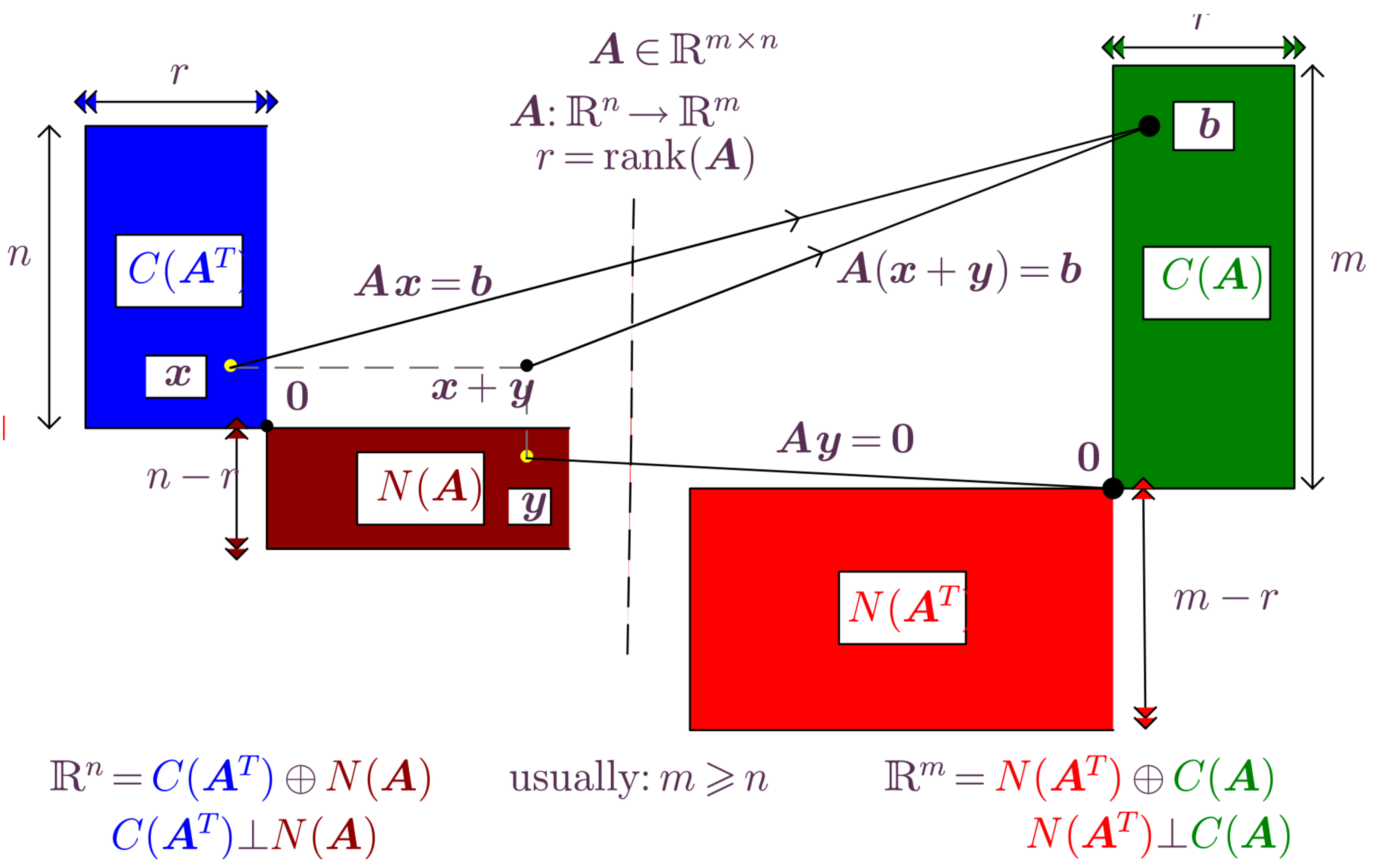
The FTLA states a decomposition of the domain and codomain of a linear mapping \(T : \mathbb{R}^n \rightarrow \mathbb{R}^m\), \(T (\boldsymbol{x}) =\boldsymbol{A}\boldsymbol{x}\).
In applications bases for the four fundamental spaces are also required. Recall that a basis a linearly independent spanning set for a vector space. In Matlab/Octave, a basis for \(C (\boldsymbol{A})\) is given by orth(A), and a basis for \(N (\boldsymbol{A})\) is givrn by null(A).
Here are some examples.
1.
The output from orth(A):
2.1615e-15 1.0000e+00 -2.0106e-16
8.1124e-01 -1.6364e-15 5.8471e-01
-5.8471e-01 1.1913e-15 8.1124e-01
Replacing small quantities with zero (inexact computer arithmetic) gives:
0 1.0000e+00 0
8.1124e-01 0 5.8471e-01
-5.8471e-01 0 8.1124e-01
There are 3 linearly independent vectors in orth(A), hence rank(A)=3, and the system \(A x = b\) has a unique solution for any \(b\). The null space \(N (A)\) should only contain the zero vector. Indeed, null(A) in Octave returns:
ans = []
Read the above as stating “there are no linearly independent vectors that span N(A)”.
2.
The output from orth(A) is
0.935113 -0.186157
0.342275 0.254295
-0.091712 -0.949041
There are now two linearly independent (column) vectors, hence rank(A)=2. By the FTLA the dimension of \(N (A)\) should be 1, and indeed null(A) now gives:
-0.5774
-0.5774
0.5774
The system \(A x = b\) has an infinite number of solutions for \(b \in C (A)\). Since vectors in orth(A) span \(C (A)\), any linear combination of these vectors gives such a \(b\), for example
If \(b\) is within \(N (A^T)\), the system does not have a solution. Compute null(transpose(A)) to obtain
-0.3015
0.9045
0.3015
Any scaling of the above vector gives a rhs for which the system has no solution.
3.
orth(A) gives
0.2534 0.9674
0.9674 -0.2534
with two linearly independent vectors, hence rank(A)=2. Computing null(A) gives
2.7997e-01 -4.3303e-01 -7.5673e-01
-8.5573e-01 -4.8086e-01 -7.0125e-03
3.0834e-01 -2.2673e-01 2.0253e-01
-2.6872e-01 6.8707e-01 -2.1040e-01
1.4855e-01 -2.4039e-01 5.8483e-01
with 3 linearly independent vectors. The system Ax=b always has an infinite number of solutions.
4.
orth(A) gives
-0.495688 -0.510213
0.264100 0.050401
-0.824813 0.258209
0.065024 -0.818823
with 2 linearly independent vectors, hence rank(A)=2.
null(transpose(A)) gives
-0.019026 -0.702577
0.930667 -0.248134
0.322906 0.385673
0.170966 0.544125
and null(A) contains only the zero vector.
For \(b = \left[ \begin{array}{l} - 0.495688\\ 0.264100\\ - 0.824813\\ 0.065024 \end{array} \right]\) the system has a unique solution, while for \(b = \left[ \begin{array}{l} - 0.019026\\ 0.930667\\ 0.322906\\ 0.170966 \end{array} \right]\) the system does not have any solution.