MATH347DS

Problem 1

Data

𝒟 = {(t_{j}, x_{j}), j = 1, 2, \dots, m}

can be represented in multiple ways. The course desribed the least squares solution to representing the data as a polynomial, for instance a quadratic polynomial

p (t) = c_{0} + c_{1} t + c_{2} t^{2}

the coefficients of which are found by solving

{min}_{𝒂 \in ℝ^{3}} || 𝒙 - 𝑨 𝒄 ||, 𝒄 = [\begin{array}{l} c_{1} \\ c_{2} \\ c_{3} \end{array}], 𝒙 = [\begin{array}{l} x_{1} \\ x_{2} \\ ⋮ \\ x_{m} \end{array}], 𝒕^{k} = [\begin{array}{l} t_{1}^{k} \\ t_{2}^{k} \\ ⋮ \\ t_{m}^{k} \end{array}], 𝑨 = [\begin{array}{lll} 𝒕^{0} & 𝒕^{1} & 𝒕^{2} \end{array}] .

(1)

Notice that

p (t)

is a linear combination of

{1, t, t^{2}}

with scaling coefficients

c_{0}, c_{1}, c_{2}

, and recall that

t_{i}^{0} = 1

Consider another representation of the data as a trigonometric polynomial $q (t) = a_{0} + a_{1} \sin (t) + a_{2} \cos (t)$ . State the least squares problem by modifying (1) to reflect the new representation.

Solution. The columns of $𝑨$ change

{min}_{𝒂 \in ℝ^{3}} || 𝒙 - 𝑨 𝒄 ||, 𝒄 = [\begin{array}{l} c_{1} \\ c_{2} \\ c_{3} \end{array}], 𝒙 = [\begin{array}{l} x_{1} \\ x_{2} \\ ⋮ \\ x_{m} \end{array}], 𝒕^{k} = [\begin{array}{l} t_{1}^{k} \\ t_{2}^{k} \\ ⋮ \\ t_{m}^{k} \end{array}], 𝑨 = [\begin{array}{lll} 𝟏 & \sin (𝒕) & \cos (𝒕) \end{array}] .

(2)

For $m = 100$ , $t_{j} = 2 π j / m$ for $j = 1, 2, \dots, m$ , arbitrarily choose some values for $a_{0}, a_{1}, a_{2} \in [- 1, 1]$ , and construct data vectors $𝒕, 𝒙 \in ℝ^{m}$ in Octave.

Solution.

octave]

m=100; t=2*pi*(1:m)'/m;

octave]

a0=-0.5; a1=0.5; a2=1.0; aEX=[a0; a1; a2];

octave]

x=a0+a1*sin(t)+a2*cos(t);

octave]

Solve in Octave the least squares problem you stated in point 1. Do you recover the coefficients $a_{0}, a_{1}, a_{2}$ you chose?

octave]

A=[t.^0 sin(t) cos(t)];

octave]

[Q,R]=qr(A,0); b=Q'*x; aLS=R\b; aLS'

ans = -0.50000 0.50000 1.00000

octave]

Coefficients are exactly recovered.

Perturb the data to mimic measurement noise $𝒚_{s} = 𝒙 + s 𝒓$ , where $𝒓$ is a vector of random numbers in the interval $[- 1, 1]$ scaled by $s = 1$ . Solve the least squares problem for the new, noisy data to obtain the perturbed coefficients $\tilde{𝒂}$ .

octave]

y = x + 2*(rand(m,1)-0.5);

octave]

b=Q'*y; aLS=R\b; aLS'

ans = -0.34031 0.50169 1.04731

octave]

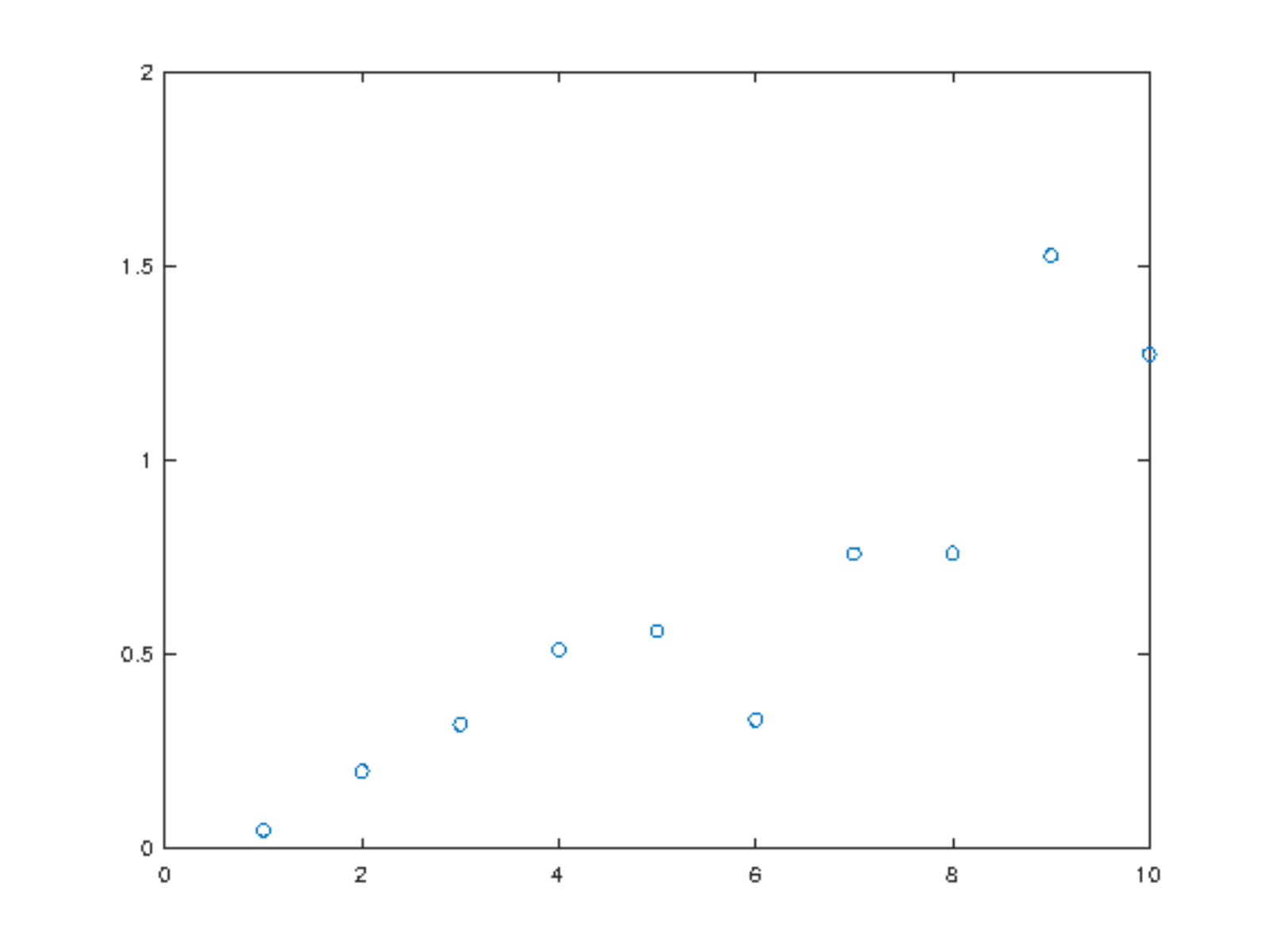
Write an Octave loop over the scaling coefficient values $s = 1, 2, \dots, n$ with $n = 10$ , and compute the norm of the change in the coefficients $e_{s} = || \tilde{𝒂} - 𝒂 ||$ for each $s$ value. Construct a plot of $(s, e_{s})$ and comment on the effect of the magnitude of the noise as measured by $s$ upon recovery of the exact coefficients $𝒂 .$

octave]

n=10; err=zeros(n,1);
for s=1:n
  y = x + 2*s*(rand(m,1)-0.5);
  b=Q'*y; aLS=R\b;
  err(s) = norm(aLS-aEX);
end

octave]

plot(1:n,err,'o')

octave]

cd ~/courses/MATH347DS; print -depsc 'errplot.eps'

octave]

Figure 1. Error $e_{s} = || 𝒂_{s} - 𝒂 ||$ grows with $s$

Problem 2

Continuing the above, suppose the measurement noise is modulated in time,

𝒚_{s} = 𝒙 + s 𝒓 \sin (𝒕) + 4 s 𝒓 \sin (2 𝒕) .

(3)

Investigate now the utility of the singular value decomposition to gain insight into the data.

Construct a data matrix of the modulated noise measurements specified in formula (3)

𝒀 = [\begin{array}{llll} 𝒚_{1} & 𝒚_{2} & \dots & 𝒚_{10} \end{array}]

octave]

n=10; Y = zeros(m,n); err=zeros(n,1);
for s=1:n
  y = x + s*2*(rand(m,1)-0.5).*sin(t) + 4*s*2*(rand(m,1)-0.5).*sin(2*t);
  Y(:,s) = y;
end

octave]

Compute the mean of the measurements $\overline{𝒚}$ , and construct the centered data matrix

𝒀_{0} = [\begin{array}{llll} 𝒚_{1} - \overline{𝒚} & 𝒚_{2} - \overline{𝒚} & \dots & 𝒚_{10} - \overline{𝒚} \end{array}]

octave]

yAV = mean(Y')'; size(yAV)

ans = 100 1

octave]

Y0=Y-yAV;

octave]

Compute the first 3 singular vectors of $𝒀_{0}$ using the svds Octave function.

octave]

[U S V]=svds(Y0,3);

octave]

The largest 10 singular values are found through the instruction sigma=svds(Y,10,'L'). Display these values and comment on your observations.

octave]

sigma=svds(Y,10,'L')'

sigma = Columns 1 through 8: 189.757 161.290 139.115 115.779 96.063 84.466 64.798 48.051 Columns 9 and 10: 31.548 16.625

octave]

Singular values decay quickly.

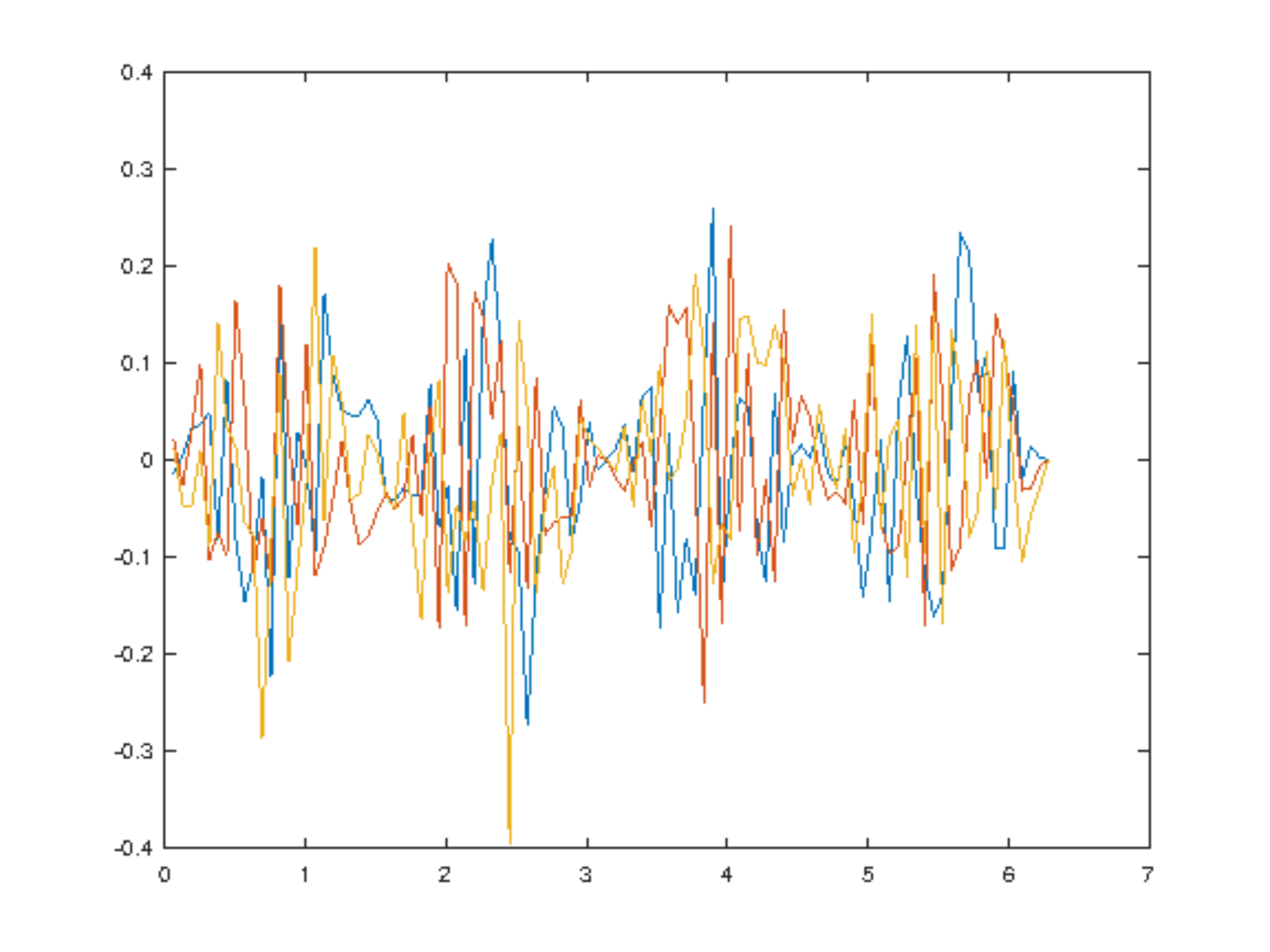
Plot the first 3 singular vectors. What features of the data $𝒀$ is revealed by the dominant singular vectors?

octave]

plot(t,U(:,1),t,U(:,2),t,U(:,3))

octave]

print -depsc 'uplot.eps'

octave]

Figure 2. The singular vectors capture the noice modulation $\sin (t), \sin (2 t)$