MATH347DS L06: Applying the FTLA (LU)

Overview

• Least squares as an application of projection and $𝑸𝑹$ factorization

• Change of coordinates (linear systems), $𝑳𝑼$ factorization

Least squares method and solution by projection

Figure 1. Least squares problem: find $𝒗\in C\left(𝑨\right)$, $𝑨\in {ℝ}^{m\times n}$ closest to some given $𝒚$ in the 2-norm

• Mathematical statement: solve the minimization problem ${min}_{𝒄\in {ℝ}^n}||𝒚-𝑨𝒄||$

• Approach: project $𝒚$ onto the column space of $𝑨$:

  1. Find an orthonormal basis for column space of $𝑨$ by $𝑸𝑹$ factorization, $𝑸𝑹=𝑨$

  2. State that $𝒗$ is the projection of $𝒚$, $𝒗={𝑷}_{C\left(𝑨\right)}𝒚={𝑷}_{𝑸}𝒚=𝑸{𝑸}^T𝒚$

  3. State that $𝒗$ is within the column space of $𝑨$, $𝒗=𝑨𝒄=𝑸𝑹𝒄$

  4. Set equal the two expressions of $𝒗$, $$$𝑸{𝑸}^T𝒚=𝑸𝑹𝒄\Rightarrow 𝑹𝒄={𝑸}^T𝒚$

  5. Solve the triangular system to find $𝒄$ (in Octave: c=R\(Q'y))

Linear regression coding

1. Generate some data on a line and perturb it by some random quantities

   octave>

   m=1000; x=(0:m-1)/m; c0=2; c1=3; yex=c0+c1*x; y=(yex+rand(1,m)-0.5)';

2. Form the $𝑸,𝑹$ matrices, $𝑸𝑹=𝑨$, (qr(A,0) is the Octave gs(A))

   octave>

   A=ones(m,2); A(:,2)=x(:); [Q R]=qr(A,0);

3. Solve the system $𝑹𝒙={𝑸}^T𝒃$

   octave>

   c=R\(transpose(Q)*y);

4. Form the linear combination $𝒗=𝑨𝒙$ closest to $𝒃$

   octave>

   v=A*c;

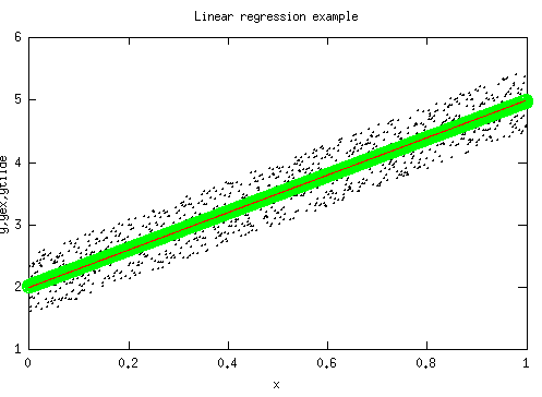
Linear regression example

• Plot the perturbed data (black dots), the result of the linear regression (green circles), as well as the line used to generate yex (red line)

  octave>

  plot(x,y,'.k',x,v,'og',x,yex,'r'); title('Linear regression example'); xlabel('x'); ylabel('y,v,yex'); cd /home/student; print data.eps;

Quadratic regression

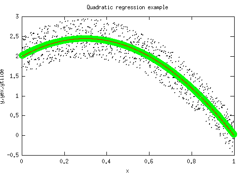
• The key observation is that the matrix $𝑨$ has columns obtained by evaluating the functions $1,x$ at the values $x_1,x_2,\dots ,x_m$. This leads to easy extension to data fitting to higher degree polynomials, for instance a quadratic

  ${\displaystyle 𝒆=\left(\begin{array}{ccc}𝟏& 𝒙& {𝒙}^2\end{array}\right)𝒄-𝒚=𝑨𝒄-𝒚,min||𝒆||\Rightarrow 𝑹𝒄={𝑸}^T𝒚}$

octave> 

m=1000; x=(0:m-1)/m; c0=2; c1=3; c2=-5.; yex=c0+c1*x+c2*x.^2; y=(yex+rand(1,m)-0.5)';

octave> 

A=ones(m,3); A(:,2)=x(:); A(:,3)=x.^2; [Q R]=qr(A,0)

octave> 

c=R\(transpose(Q)*y);

octave> 

v=A*c; disp(c');

octave> 

disp(norm(y-v)/norm(y)/m);

octave> 

Quadratic regression example

• Plot the perturbed data (black dots), the result of the quadratic regression (green circles), as well as the parabola used to generate yex (red line)

octave> 

plot(x,y,'.k',x,ytilde,'og',x,yex,'r'); title('Quadratic regression example'); xlabel('x'); ylabel('y,yex,ytilde'); cd /home/student; print data.eps;

octave> 

The $m=n$ case: polynomial interpolation

Definition. The polynomial interpolant of data $𝒟=\{(x_i,y_i),i=1,\dots ,m\}$ with $x_i\ne x_j$ if $i\ne j$ is a polynomial of degree $m-1$

that satisfies the conditions $p_{m-1}\left(x_i\right)=y_i$, $i=1,\dots ,m$.

• We can apply the same approach. In this particular case, the error $𝒆$ can be made zero.

octave> 

m=4; x=(0:m-1)'; c0=2; c1=3; c2=-5.; c3=-1; y=c0+c1*x+c2*x.^2+c3*x.^3;

octave> 

A=ones(m,m); A(:,2)=x(:); A(:,3)=x.^2; A(:,4)=x.^3; [Q R]=qr(A,0);

octave> 

c=R\(transpose(Q)*y); disp(c');

Note that the coefficients used to generate the data are recovered exactly.

Gaussian elimination

• Recall the basic operation in row echelon reduction: constructing a linear combination of rows to form zeros beneath the main diagonal, e.g.

  ${\displaystyle 𝑨=\left(\begin{array}{cccc}{a}_{11}& a_{12}& \dots & a_{1m}\\ a_{21}& a_{22}& \dots & a_{2m}\\ a_{31}& a_{32}& \dots & a_{3m}\\ ⋮& ⋮& \ddots & ⋮\\ a_{m1}& a_{m2}& \dots & a_{mm}\end{array}\right)\sim \left(\begin{array}{cccc}{a}_{11}& a_{12}& \dots & a_{1m}\\ 0& a_{22}-\frac{a_{21}}{a_{11}}{a}_{12}& \dots & a_{2m}-\frac{a_{21}}{a_{11}}{a}_{1m}\\ 0& a_{32}-\frac{a_{31}}{a_{11}}{a}_{12}& \dots & a_{3m}-\frac{a_{31}}{a_{11}}{a}_{1m}\\ ⋮& ⋮& \ddots & ⋮\\ 0& a_{m2}-\frac{a_{m1}}{a_{11}}{a}_{12}& \dots & a_{mm}-\frac{a_{m1}}{a_{11}}{a}_{1m}\end{array}\right)}$

• This can be stated as a matrix multiplication operation, with $l_{i1}=a_{i1}/a_{11}$

  ${\displaystyle \left(\begin{array}{cccc}1& 0& \dots & 0\\ -l_{21}& 1& \dots & 0\\ -l_{31}& 0& \dots & 0\\ ⋮& ⋮& \ddots & ⋮\\ -l_{m1}& 0& \dots & 1\end{array}\right)\left(\begin{array}{cccc}{a}_{11}& a_{12}& \dots & a_{1m}\\ a_{21}& a_{22}& \dots & a_{2m}\\ a_{31}& a_{32}& \dots & a_{3m}\\ ⋮& ⋮& \ddots & ⋮\\ a_{m1}& a_{m2}& \dots & a_{mm}\end{array}\right)=\left(\begin{array}{cccc}{a}_{11}& a_{12}& \dots & \\ 0& a_{22}-l_{21}{a}_{12}& \dots & \\ 0& a_{32}-l_{31}{a}_{12}& \dots & \\ ⋮& ⋮& \ddots & \\ 0& a_{m2}-l_{m1}{a}_{12}& \dots & \end{array}\right)}$

Gauss multiplier

Definition. The matrix

with $l_{i,k}=a_{i,k}^{\left(k\right)}/a_{k,k}^{\left(k\right)}$, and ${𝑨}^{\left(k\right)}=\left(a_{i,j}^{\left(k\right)}\right)$ the matrix obtained after step $k$ of row echelon reduction (or, equivalently, Gaussian elimination) is called a Gaussian multiplier matrix.

Matrix formulation of Gaussian elimination

• For $𝑨\in {ℝ}^{m\times m}$ nonsingular, the successive steps in row echelon reduction (or Gaussian elimination) correspond to successive multiplications on the left by Gaussian multiplier matrices

  ${\displaystyle {𝑳}_{m-1}{𝑳}_{m-2}\dots {𝑳}_2{𝑳}_1𝑨=𝑼}$

• The inverse of a Gaussian multiplier is

  ${\displaystyle {𝑳}_k^{-1}=\left(\begin{array}{ccccc}1& \dots & 0& \dots & 1\\ 0& \ddots & 0& \dots & 0\\ 0& \dots & 1& \dots & 0\\ 0& \dots & l_{k+1,k}& \dots & 0\\ 0& \dots & l_{k+2,k}& \dots & 0\\ ⋮& \dots & ⋮& \ddots & ⋮\\ 0& \dots & l_{m,k}& \dots & 1\end{array}\right)=𝑰-({𝑳}_k-𝑰)}$

$𝑳𝑼$ factorization

• From $\left({𝑳}_{m-1}{𝑳}_{m-2}\dots {𝑳}_2{𝑳}_1\right)𝑨=𝑼$ obtain

  ${\displaystyle 𝑨={\left({𝑳}_{m-1}{𝑳}_{m-2}\dots {𝑳}_2{𝑳}_1\right)}^{-1}𝑼={𝑳}_1^{-1}{𝑳}_2^{-1}\cdot \dots \cdot {𝑳}_{m-1}^{-1}𝑼=𝑳𝑼}$

• Due to the simple form of ${𝑳}_k^{-1}$ the matrix $𝑳$ is easily obtained as

  ${\displaystyle 𝑳=\left(\begin{array}{cccccc}1& 0& 0& \dots & 0& 0\\ l_{2,1}& 1& 0& \dots & 0& 0\\ l_{3,1}& l_{3,2}& 1& \dots & 0& 0\\ ⋮& ⋮& ⋮& \ddots & ⋮& ⋮\\ l_{m-1,1}& l_{m-1,2}& l_{m-1,3}& \dots & 1& 0\\ l_{m,1}& l_{m,2}& l_{m,3}& \dots & l_{m,m-1}& 1\end{array}\right)}$

Solving a linear system by $L𝑼$ factorization

• Using the concept of an $𝑳𝑼$ factorization, finding the solution to a linear system $𝑨𝒙=𝒃$ can be formulated as the following steps:

  1. Find the $𝑳𝑼$ factorization, $𝑳𝑼=𝑨$

  2. Replace factorization into system and regroup $𝑨𝒙=𝒃\iff (𝑳𝑼)𝒙=𝒃\iff 𝑳𝒚=𝒃$. Solve the lower triangular $𝑳𝒚=𝒃$ system to find $𝒚$

  3. Solve the upper triangular system $𝑼𝒙=𝒚$ to find $𝒙$