1.MATH347 Homework 4

1.1.Background

The final linear algebra problem investigated in the course is finding invariant directions for a homogeneous linear mapping $𝒇:{ℂ}^m\to {ℂ}^m$, $𝒇\left(𝒙\right)=𝑨𝒙$, known as the eigenproblem

It is known that $m$ eigenvalues and associated eigenvectors exist to satisfy the above relation $𝑨{𝒙}_i={\lambda }_i{𝒙}_i$, $i=1,\dots ,m$, and the eigenproblem can be stated in matrix form as

1.2.Theoretical questions

1. Write the rotation matrix ${𝑹}_{\theta }$ of angle $\theta$ around axis ${𝒆}_3\in {ℝ}^3$. Find the eigenvalues and eigenvectors of $R_{\theta }.$ (1 point)

2. Find a matrix $𝑨\ne 𝟎$ for which ${𝑨}^3=0$. What are the eigenvalues of $𝑨$?(2 points)

3. If $𝑩\in {ℝ}^{3\times 3}$ has eigenvalues 0,1,2 give values (or state that there is not enough information to specify a value) for:

   1. rank$\left(B\right)$

   2. eigenvalues of $B^{T}B$

   3. eigenvalues of ${(B^2+I)}^{-1}$

   (3 points)

4. Determine the singular value decomposition and pseudo-inverse of a matrix $𝑨\in {ℝ}^{1\times n}$ (i.e., a row vector). (2 points)

1.3.Molecular Eigenmodes

1.3.1.Introduction

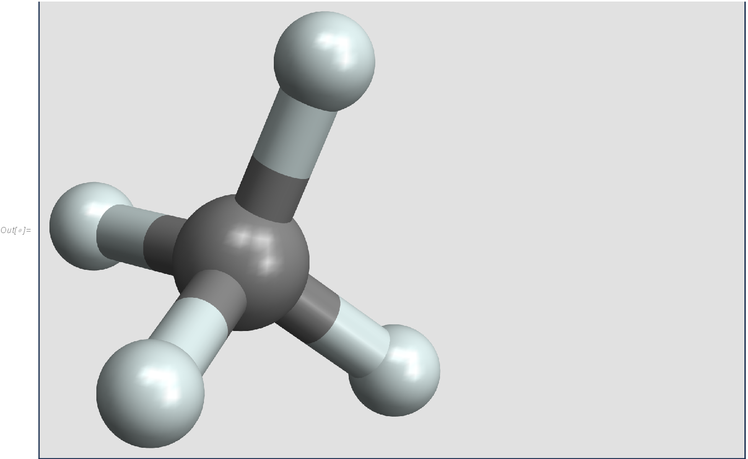
Molecules are composed from atoms interacting through electromagnetic forces generated by their electron orbital shells. The methane molecule ${\mathrm{CH}}_4$ contains a carbon atom and four hydrogen atoms

Figure 1. Methane molecule

The positions of the methane atoms are given in Table 1.

Molecular properties are largely determined by the vibration of the atoms around equilibrium positions. The equilibrium configuration of the methane molecule can be expressed through a single vector $𝒛\in {ℝ}^{15}$

with $𝒙$ vectors from Table 1 for the carbon and four hydrogen atoms.

∴ 

Z=[0 0 0; -0.13066  -1.02319 0.359047; -0.713551 0.656267 0.503049; 1.01707   0.334488 0.215849; -0.172858 0.032433 -1.07795];

∴ 

fig=figure();

∴ 

ax = fig.add_subplot(projection="3d");

∴ 

ax.scatter(Z[1,1],Z[1,2],Z[1,3],color="black");

∴ 

ax.scatter(Z[2:5,1],Z[2:5,2],Z[2:5,3],color="red");

∴ 

ax.plot(Z[1:2,1],Z[1:2,2],Z[1:2,3],color="blue");

∴ 

ax.plot(Z[1:2:3,1],Z[1:2:3,2],Z[1:2:3,3],color="blue");

∴ 

ax.plot(Z[1:3:4,1],Z[1:3:4,2],Z[1:3:4,3],color="blue");

∴ 

ax.plot(Z[1:4:5,1],Z[1:4:5,2],Z[1:4:5,3],color="blue");

∴ 

Vibration around this equilibrium position is described by a displacement vector $𝒖\in {ℝ}^{15}$ such that the position of the atoms is $𝒚=𝒛+𝒖$. The displacement vectors are known as vibrational eigenmodes and are determined by the eigenproblem

The matrix $𝑨$ is symmetric $𝑨={𝑨}^T$, captures chemical bond strengths between the atoms and has a block structure

with diagonal blocks ${𝑨}_{ii}=𝑰$ for $i=1,\dots ,5$, and off-diagonal blocks ${𝑨}_{ij}=-𝑰$ if there is a bond between atoms $i,j$, and ${𝑨}_{ij}=𝟎$ if there is no bond. The inertia matrix $𝑴$ is block diagonal

with $m_C=12$, $m_H=1$.

1.3.2.Tasks

1. Form the $𝑨,𝑴$ matrices in Julia. Compute $𝑩={𝑴}^{-1}𝑨$. Note that

   ${\displaystyle {𝑴}^{-1}=\left[\begin{array}{lllll}{m}_C^{-1}𝑰& & & & \\ & m_H^{-1}𝑰& & & \\ & & m_H^{-1}𝑰& & \\ & & & m_H^{-1}𝑰& \\ & & & & m_H^{-1}𝑰\end{array}\right]}$

2. Compute the eigenvalues of $𝑩$.

3. Compute the eigenvectors $𝒖$ of $𝑩$.

4. Plot the vibrational modes by plotting the equilibrium positions $𝒛$ and the vibration mode $𝒛+\alpha 𝒖$ with $\alpha$ arbitrarily chosen to ensure visibility.