Scientific Writing and Computation

Linear algebra is an excellent discipline to introduce mathematical notation, statements, abstraction, proof techniques, scientific writing and computation. This preamble to the Linear Algebra for Data Science Applications course provides a succint primer on the above.

1.Mathematical notation

Everyday shopping experience at a supermarket would suggest that tomatoes are a “vegetable” in the same group as carrots, spinach, or broccoli. The conundrum of whether tomatoes are a “vegetable” or a “fruit” provides opportunity for light-hearted socialization. In contrast to such social interaction, science imposes precise, immutable definitions. Upon defining vegetables as parts of plants consumed by humans, with those parts including seeds, fruits, flowers, leaves, stems and roots, more precise classification is possible. Tomatoes are indeed vegetables, since they are consumed by humans. Upon further defining a “fruit” as the seed-bearing part of a plant developing from a flower, it is established that tomatoes are fruits.

The above discussion is an example of the transition from casual language to scientific statements. What is lost in social interaction among humans is gained in clarity of expression and lays the basis for modifying Nature, for instance in the case of plants by cultivation techniques. It is however dependent on a particular natural language (English), and somewhat long-winded. A key feature of mathematics is the introduction of a precise and succint language and associated notation. Even though the full language contains many constructs, a few basic constructs are repeatedly encountered and should be mastered. These constructs are introduced gradually throughout this course as needed, but a first collection includes the following.

Sets

A set is a collection of objects, for example,

${\displaystyle \mathrm{digits}=\{0,1,2,3,4,5,6,7,8,9\}.}$

(1)

In natural language the above is read as: “digits is a set containing 0,1,2,3,4,5,6,7,8,9”. It is important to note several aspects of the above rather mundane expression. Formula (1) contains several notations: “=” for denoting equality, “$\left\{\right\}$” to denote a collection. Instead of the word “digits” a shorter symbol, say $𝒟$, could be used

${\displaystyle 𝒟=\{0,1,2,3,4,5,6,7,8,9\}.}$

(2)

When it is clear from context, not all members of the set need be listed

${\displaystyle 𝒟=\{0,1,\dots ,9\}.}$

(3)

The fact that “3” is a digit is stated as

${\displaystyle 3\in 𝒟,}$

(4)

read as “3 is a member of the set of digits”, with the symbol “$\in$” denoting membership. Smaller collections can be included in larger ones such as the statement “all even digits are digits”, expressed as

${\displaystyle \{0,2,4,6,8\}\subset \{0,1,2,3,4,5,6,7,8,9\},}$

(5)

where the inclusion symbol “$\subset$” has been introduced. Introducing a notation for the even digits $ℰ=\{0,2,4,5,6,8\}$ allows a more concise form of (5)

${\displaystyle ℰ\subset 𝒟.}$

The fact a set can include itself can be stated through the “$\subseteq$” symbol, as in

${\displaystyle 𝒟\subseteq 𝒟.}$

Formulas

Once mathematical symbols have been introduced, combinations of such symbols can be constructed. The combination of symbols has meaning if the symbols can be interpreted, either by a human or a computer. Using the symbols “3”, “$\in$”, “$𝒟$” introduced above the combinations

${\displaystyle \begin{array}{lll}𝒟\in 3,& 𝒟3\in ,& \in 𝒟3,\\ \in 3𝒟,& 3𝒟\in ,& 3\in 𝒟,\end{array}}$

can be formed. They could be read as:

digits belongs to three,	digits three belongs to,	belongs to digits three,
belongs to three digits,	three digits belongs to,	three belongs to digits.

Irrespective of the Yoda-like interpretations that can be given, only the last statement can be meaningfully interpreted. Such meaningful sequences of symbols are known as formulas. The symbols in (2) constitute a formula that defines the symbol $𝒟$.

Quantifiers

Within formulas some symbols may have a single meaning such as in $1+1=2$, where the symbols “1”, “+”, “=”, “2” are all uniquely defined. Other formulas may contain symbols with multiple meanings such as “$x+y=2$”, in which the symbols $x$, $y$ are known as variables. It is useful to have a means to specify how many instances of the variables statisfy some formula. This is accomplished through quantifiers:

For any, $\forall$

A variable can take any value from within a set, $\forall x\in \{1,2,3\}:2x\in ℰ$, read as “for any $x$ value chosen from 1,2,3, twice $x$ is an even”.

There exists, $\exists$

There is some value within a set, $\exists x\in 𝒟:x\in ℰ$, read as “there exists some digit which is even”.

There exists only one, $\exists !$

There is only one value within a set, $\exists !x\in 𝒟$: $2x=4$, read as “there is only one digit, twice of which is equal to four”.

2.Mathematical statements

An English sentence is a complete unit of thought containing a subject, a verb, perhaps an object. The following are examples of English sentences:

A contrast can be made to:

none of which are sentences.

Formula (1) is a mathematical statement, similar to an English sentence. The following is a counter example to (1)

Careful study of the displayed symbols would perhaps lead to the natural language reading “digits collection of 0,1,2,3,4,5,6,7,8,9”. No relationship is however stated between “digits” and the numbers within the collection; the symbols in (6) do not form a mathematical statement nor a natural language sentence since the verb is missing. Just as a sentence in English contains punctuation, so does the mathematical statement (1) include a period at the end to denote the end of the statement. In contrast perhaps to English sentence, a mathematical statement must be ascertainable as either true (T) or false (F).

Compound mathematical statements can be formed by connectives: the conjunction (AND, $\wedge$), the disjunction (OR, $\vee$), negation (NOT, $\neg$), conditionals (IF $A$ THEN $B$, $A\Rightarrow B$), and biconditionals ($A$ IF AND ONLY IF $B$, $A\iff B$). The truth of compound mathematical statements is conveniently stated through truth tables.

Mathematical statement subjects can refer to a single entity (constants) or multiple entities (variables). All the following are well formed mathematical statements even though the third one is false

Some common mathematics verbs are:

The imply verb is used as in $A\Rightarrow B$ and states that from truth of statement $A$, the truth of statement $B$ results. The equivalent verb is a bi-directional imply, in that $A\iff B$ has the same meaning as $A\Rightarrow B$ and $B\Rightarrow A$.

3.Mathematical abstraction

Mathematics concentrates on recognizing relationships between groups of objects. A familiar example is quantification, recognition of the abstract concept of number. The two sets $A=${Mary, Jane, Tom} and $B=${apple, plum, cherry} seem quite different, but we can match one distinct person to one distinct fruit as in {Mary$\leftrightarrow$plum, Jane$\leftrightarrow$apple, Tom$\leftrightarrow$cherry}. There is an abstraction that can be attached to both sets, that of the number “3”. Algebra is the branch of mathematics that defines precise rules to work with mathematical statements. This is accomplished by defining sets of objects to work with and operations between elements of the sets. A familiar case is abstraction of the process of counting by introducing the set of natural numbers $\mathbb{N}=\{0,1,2,3,\dots \}$ and the addition operation $+$ . Example additions are $1+1=2$, $2+3=5$. It is impossible to explicitly list all additions, so mathematical statements using quantifiers are used to define the following rules:

Closure

$\forall a,b\in \mathbb{N}:a+b\in \mathbb{N}$. Adding two naturals results in a natural.

Associativity

$\forall a,b,c\in \mathbb{N}:(a+b)+c=a+(b+c)$. Adding the first two naturals to a third is the same as adding the first to the sum of the last two naturals.

Commutativity

$\forall a,b\in \mathbb{N}:a+b=b+a$. Adding a first natural to a second is the same as adding the second to the first.

Identity

$\exists 0\in \mathbb{N}:\forall a\in N:a+0=a$. There exists a special natural, the identity element, denoted as 0, such that when added to any natural the result is the chosen natural.

Comparison of the rather long English sentences to the concise mathematical statements highlights the utility of formalized notation.

4.Proof techniques

Establishing the truth value of a mathematical statement is akin to an art form, requiring practice, insight and technical mastery. Nonetheless, some common techniques are readily grasped and of great value in applying mathematics to practical problems.

Direct proofs

Starting from statements known to be true (definitions, axioms, previously proven statements), form combinations of these statements.

Example

$S:$ Sum of even naturals (the set $ℰ$) is even. Use definition of even $E:x\in ℰ\Rightarrow \exists a\in \mathbb{N}:x=2a=a+a$. Again use definition of even $E:y\in ℰ\Rightarrow \exists b\in \mathbb{N}:y=2b=b+b$. Use definition of addition, $x+y=a+a+b+b$. Use commutativity, $x+y=a+b+a+b=2(a+b)$, and establish result by definition of even, $x+y\in ℰ$. This proof is concisely stated in mathematical notation as

${\displaystyle x,y\in ℰ\Rightarrow \exists a,b\in \mathbb{N}:x=2a\wedge y=2b\Rightarrow x+y=2(a+b)\in ℰ\square .}$

Proof by induction

If a natural number $n$ can be identified within some mathematical statement $P$, establish a sequence of true statements for $n=1,2,\dots$. In practice, the statement is proven for a small value of $n$, $P\left(1\right)$, and then from assuming $P\left(n\right)$ true a proof is sought for $P(n+1)$. The statement is thereby established for all natural numbers.

Example

$S\left(n\right):\forall n\in \mathbb{N}:2n\in ℰ$, all natural numbers $2n=n+n$ are even. First, state $S\left(1\right):2\in ℰ$, which is true. Next, assume $S\left(n\right)$ is true, $2n\in ℰ$. Then $S(n+1):2(n+1)\in ℰ$, is true by definition.

Proof by contrapositive

When seeking to prove the statement $S:P\Rightarrow C$, that from premise $P$ the conclusion $C$ results, proof by contrapositive seeks to prove that negation of the conclusion implies negation of the premise, $\neg C\Rightarrow \neg P$. The following table establishes that the two procedures have the same truth values

$\begin{array}{llllll}P& \neg P& C& \neg C& P\Rightarrow C& \neg C\Rightarrow \neg P\\ T& F& T& F& T& T\\ T& F& F& T& F& F\\ F& T& T& F& T& T\\ F& T& F& T& T& T\end{array}$

Proof by contrapositive truth table.

Example

$S:n\in \mathbb{N}\Rightarrow 2n\in ℰ$. Contrapositive is $T:2n\notin ℰ\Rightarrow n\notin \mathbb{N}$. If $2n$ is not even, then it is odd so it can be written as $2n=2p+1$ for some $p\in \mathbb{N}$. But it then results that $n=p+1/2\notin \mathbb{N}$.

Proof by contradiction

Though one of the conceptually more non-intuitive techniques, proof by contradiction is soundly based upon truth tables. First it is useful to formally define “always true” statements and “always false” statements. These are called tautologies ($C\vee \neg C$, $C$ or not $C$) and contradictions ($C\wedge \neg C$, $C$ and not $C$) , respectively and have the following truth tables.

$\begin{array}{llll}C& \neg C& C\vee \neg C& C\wedge \neg C\\ T& F& T& F\\ F& T& T& F\end{array}$

Tautology, contradiction truth tables.

Example

$C:n\in ℰ$ (n is even). $\neg C:n\notin ℰ$ ($n$ is not even). Tautology: it is always true that $n$ is either even or not even (odd). Contradiction: it cannot be true that $n$ is both even and not even.

When seeking to prove the statement $S:P\Rightarrow C$, proof by contradiction starts by assuming the opposite conclusion arises $P\wedge \neg C$ ($P$ and not $C$). It is then sought to derive a contradiction, $P\wedge \neg C\Rightarrow C\wedge \neg C$,

$\begin{array}{lllllll}P& C& \neg C& P\Rightarrow C& P\wedge \neg C& C\wedge \neg C& P\wedge \neg C\Rightarrow C\wedge \neg C\\ T& T& F& T& F& F& T\\ T& F& T& F& T& F& F\\ F& T& F& T& F& F& T\\ F& F& T& T& F& F& T\end{array}$

Proof by contradiction truth table. Compare the truth values of the $P\Rightarrow C$ column with that of the $P\wedge \neg C\Rightarrow C\wedge \neg C$ column.

Example

$S:n\in \mathbb{N}\Rightarrow 2n\in ℰ$. Assume the opposite conclusion, that $n\in \mathbb{N}$ implies $2n\notin ℰ$. Obtain the contradiction that $2n\in ℰ$ and $2n\notin ℰ$, $2n$ cannot be both even and not even.

5.Scientific writing and computation

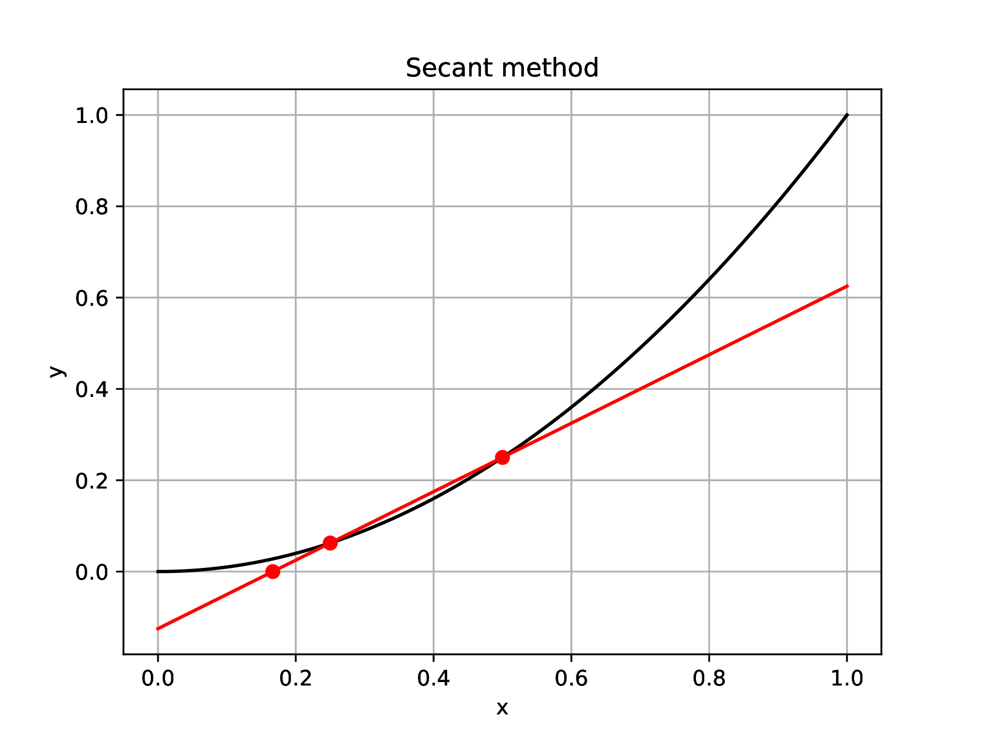
Scientific writing concentrates on precise formulation of the problem being solved, the method of study, and the conclusions of the study. Within the quantitative sciences, scientific writing typically involves intertwining English sentences, mathematical statements, computer code implementing some method of study, and graphical presentation of the conclusions of the study. Scientific text editing is eased by appropriate tools that integrate all the above facets. TeXmacs is such a scientific editing platform. It has the added benefit of being public domain software that will execute on all widely used platforms (Windows, MacOS, Linux). It allows the production of “live” documents in which students can immediately experiment with mathematical concepts presented in the document. This document is written in TeXmacs, and a simple example is plotting the intersection of the secant to a function graph with the horizontal axis. Let $f:ℝ\to ℝ$ be the function, and $(x_0,f\left(x_0\right))$, $(x_1,f\left(x_1\right))$ the points at which to construct the secant. The secant is the line passing through these two points and therefore has slope

Since the secant passes through point $(x_1,f\left(x_1\right))$, it has equation

The intersection of the secant $y\left(x\right)$ with the $x$-axis occurs when $y=0$, say at position $x_2$ along the $x$-axis leading to the equation

The above is a precise algebraic solution of the problem, but comprehension is aided by providing specific examples of $f\left(x\right)$ and resulting plots. This typically requires use of some programming language, such as the Julia language used in this course. TeXmacs allows direct insertion of Julia instructions to create “live” documents.

∴ 

f(x)=x^2; x0=0.5; x1=0.25;

∴ 

f0=f(x0); f1=f(x1); m=(f1-f0)/(x1-x0); x2=x1-f1/m;

∴ 

x=0:0.01:1; fx=f.(x); yx=m .* (x .- x1) .+ f1;

∴ 

clf(); plot(x,fx,"k",x,yx,"r",[x0 x1 x2],[f0 f1 0],"ro");

∴ 

grid("on"); xlabel("x"); ylabel("y"); title("Secant method");

∴ 

cd(homedir()*"/courses/MATH347DS/images");

∴ 

savefig("L00Fig01.eps");

∴ 

Figure 1. Secant method plot.

It is straightforward to generate new plots by changing the values of $x_0,x_1$ or the definition of the function $f\left(x\right)$.