MATH347DS

Synopsis. Data science arises from the need to organize massive amounts of data into meaningful insights into some natural or social process. There are many ways to do so such as lists, trees, clusters. Linear algebra concentrates on grouping quantifiable data into sets of fixed length, known as vectors. Multiple vectors are subsequently grouped as matrices, and a formalism is established to work with vectors and matrices.

1.Numbers

1.1.Number sets

Several types of numbers have been introduced in mathematics to express different types of quantities, and the following will be used throughout this text:

$ℕ$: The set of natural numbers, $ℕ = {0, 1, 2, 3, \dots}$ , infinite and countable, $ℕ_{+} = {1, 2, 3, \dots}$ ;
$ℤ$: The set of integers, $ℤ = {0, \pm 1, \pm 2, \pm 3, \dots}$ , infinite and countable;
$ℚ$: The set of rational numbers $ℚ = {p / q, p \in ℤ, q \in ℕ_{+}}$ , infinite and countable;
$ℝ$: The set of real numbers, infinite, not countable, can be ordered;
$ℂ$: The set of complex numbers, $ℂ = {x + i y, x, y \in ℝ}$ , infinite, not countable, cannot be ordered.

These sets of numbers form a hierarchy, with $ℕ \subset ℤ \subset ℚ \subset ℝ \subset ℂ$ . The size of a set of numbers is an important aspect of its utility in describing natural phenomena. The set $S = {Mary, Jane, Tom}$ has three elements, and its size is defined by the cardinal number, $| S | = 3$ . The sets $ℕ, ℤ, ℚ, ℝ, ℂ$ have an infinite number of elements, but the relation

z = {\begin{cases} - n / 2 & for n even \\ (n + 1) / 2 & for n odd \end{cases} .

defines a one-to-one correspondence between $n \in ℕ$ and $z \in ℤ$ , so these sets are of the same size denoted by the transfinite number $ℵ_{0}$ (aleph-zero). The rationals can also be placed into a one-to-one correspondence with $ℕ$ , hence

| ℕ | = | ℤ | = | ℚ | = ℵ_{0} .

In contrast there is no one-to-one mapping of the reals to the naturals, and the cardinality of the reals is $| ℝ | = 𝔠$ (Fraktur-script c). Intuitively, there are exponentially more reals than naturals, formally stated in set theory as $𝔠 = 2^{ℵ_{0}}$ .

1.2.Quantities described by a single number

The above numbers and their computer approximations are sufficient to describe many quantities encountered in applications. Typical examples include:

the position $x \in ℝ$ of a point on the unit line segment $[0, 1]$ , approximated by the floating point number $\tilde{x} \in 𝔽$ , to within machine epsilon precision, $| x - \tilde{x} | ⩽ ϵ$ ;
the measure of resistance to change of the rate of motion known as mass, $m \in ℝ$ , $m > 0$ ;
the population of a large community expressed as a float $p \in 𝔽$ , even though for a community of individuals the population is a natural number, as in “the population of the United States is $p = 328.2 E6$ , i.e., 328.2 million”.

In most disciplines, there is a particular interest in comparison of two quantities, and to facilitate such comparison a common reference is used known as a standard unit. For measurement of a length $L$ , the meter $ℓ = 1 m$ is a standard unit, as in the statement $L = 10 m$ , that states that $L$ is obtained by taking the standard unit ten times, $L = 10 ℓ$ . The rules for carrying out such comparisons are part of the definition of real and rational numbers.

1.3.Quantities described by multiple numbers

Other quantities require more than a single number. The distribution of population in the year 2000 among the alphabetically-ordered South American countries (Argentina, Bolivia,..,Venezuela) requires 12 numbers. These are placed together in a list known in mathematics as a tuple, in this case a 12-tuple $P = (p_{1}, p_{2}, \dots, p_{12})$ , with $p_{1}$ the population of Argentina, $p_{2}$ that of Bolivia, and so on. An analogous 12-tuple can be formed from the South American populations in the year 2020, say $Q = (q_{1}, q_{2}, \dots, q_{12})$ . Note that it is difficult to ascribe meaning to apparently plausible expressions such as $P + Q$ since, for instance, some people in the 2000 population are also in the 2020 population, and would be counted twice.

2.Vectors

2.1.Vector spaces

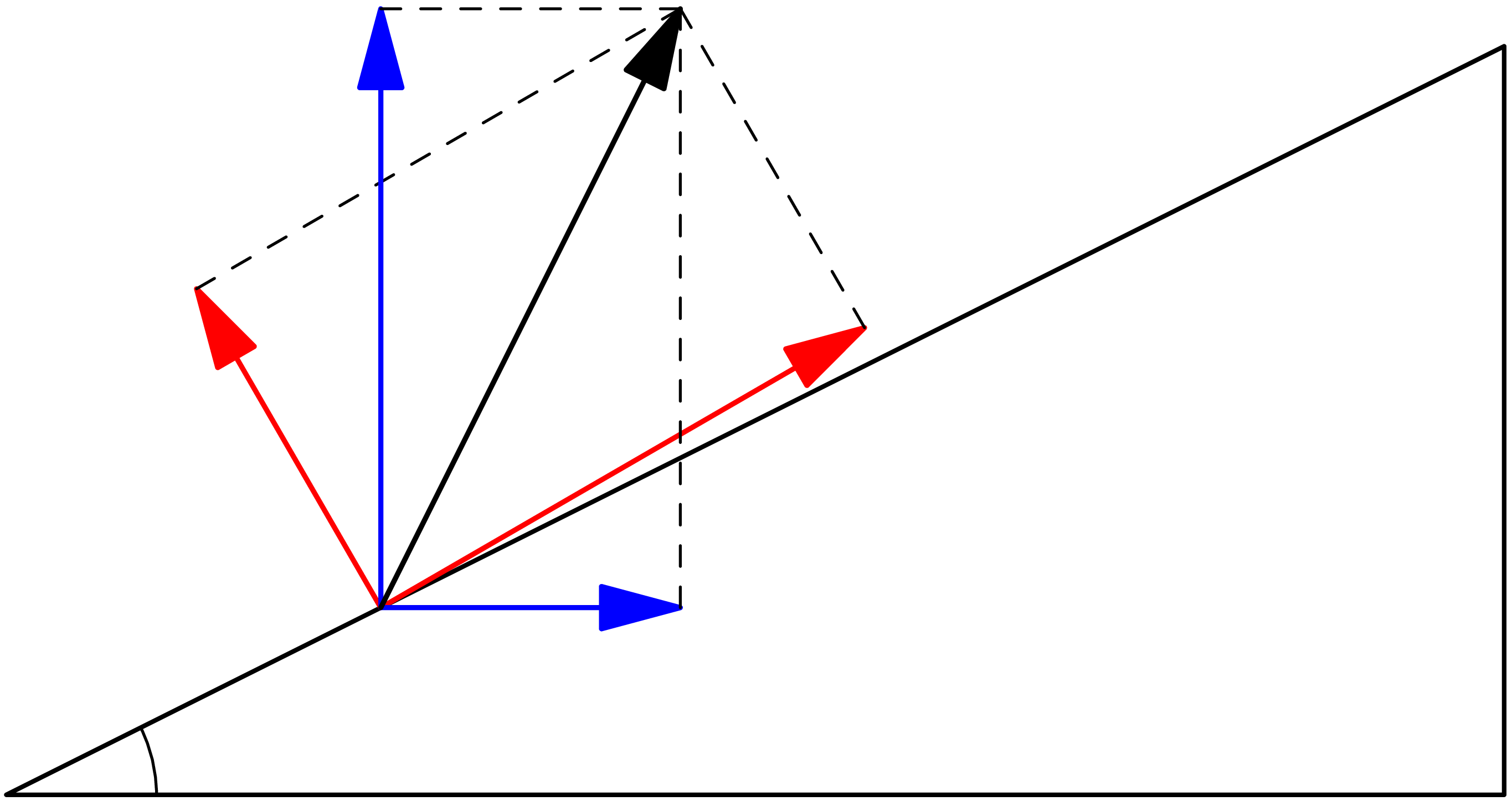
In contrast to the population 12-tuple example above, combining multiple numbers is well defined in operations such as specifying a position within a three-dimensional Cartesian grid, or determining the resultant of two forces in space. Both of these lead to the consideration of 3-tuples or triples such as the force $(f_{1}, f_{2}, f_{3})$ . When combined with another force $(g_{1}, g_{2}, g_{3})$ the resultant is $(f_{1} + g_{1}, f_{2} + g_{2}, f_{3} + g_{3})$ . If the force $(f_{1}, f_{2}, f_{3})$ is amplified by the scalar $α$ and the force $(g_{1}, g_{2}, g_{3})$ is similarly scaled by $β$ , the resultant becomes

α (f_{1}, f_{2}, f_{3}) + β (g_{1}, g_{2}, g_{3}) = (α f_{1}, α f_{2}, α f_{3}) + (β g_{1}, β g_{2}, β g_{3}) = (α f_{1} + β g_{1}, α f_{2} + β g_{2}, α f_{3} + β g_{3}) .

It is useful to distinguish tuples for which scaling and addition is well defined from simple lists of numbers. In fact, since the essential difference is the behavior with respect to scaling and addition, the focus should be on these operations rather than the elements of the tuple.

The above observations underlie the definition of a vector space $𝒱$ by a set $V$ whose elements satisfy scaling and addition properties, denoted all together by the 4-tuple $𝒱 = (V, S, +, \cdot)$ . The first element of the 4-tuple is a set whose elements are called vectors. The second element is a set of scalars, and the third is the vector addition operation. The last is the scaling operation, seen as multiplication of a vector by a scalar. Vector addition and scaling operations must satisfy rules suggested by positions or forces in three-dimensional space, which are listed in Table 1. In particular, a vector space requires definition of two distinguished elements: the zero vector $𝟎 \in V$ , and the identity scalar element $1 \in S$ .

Addition rules for	$\forall 𝒂, 𝒃, 𝒄 \in V$
$𝒂 + 𝒃 \in V$	Closure
$𝒂 + (𝒃 + 𝒄) = (𝒂 + 𝒃) + 𝒄$	Associativity
$𝒂 + 𝒃 = 𝒃 + 𝒂$	Commutativity
$𝟎 + 𝒂 = 𝒂$	Zero vector
$𝒂 + (- 𝒂_{}) = 𝟎$	Additive inverse
Scaling rules for	$\forall 𝒂, 𝒃 \in V$ , $\forall x, y \in S$
$x 𝒂 \in V$	Closure
$x (𝒂 + 𝒃) = x 𝒂 + x 𝒃$	Distributivity
$(x + y) 𝒂 = x 𝒂 + y 𝒂$	Distributivity
$x (y 𝒂) = (x y) 𝒂$	Composition
$1 𝒂 = 𝒂$	Scalar identity

Table 1. Vector space $𝒱 = (V, S, +, \cdot)$ properties.

The definition of a vector space reflects everyday experience with vectors in Euclidean geometry, and it is common to refer to such vectors by descriptions in a Cartesian coordinate system. For example, a position vector $𝒓$ within the plane can be referred through the pair of coordinates $(x, y)$ . This intuitive understanding can be made precise through the definition of a vector space $ℛ_{2} = (ℝ^{2}, ℝ, +, \cdot)$ , called the real 2-space. Vectors within $ℛ_{2}$ are elements of $ℝ^{2} = ℝ \times ℝ = {(x, y) | . x, y \in ℝ}$ , meaning that a vector is specified through two real numbers, $𝒓 \leftrightarrow (x, y)$ . Addition of two vectors, $𝒒 \leftrightarrow (s, t)$ , $𝒓 \leftrightarrow (x, y)$ is defined by addition of coordinates $𝒒 + 𝒓 = (s + x, t + v)$ . Scaling $𝒓 \leftrightarrow (x, y)$ by scalar $a$ is defined by $a 𝒓 \leftrightarrow (a x, a y)$ . Similarly, consideration of position vectors in three-dimensional space leads to the definition of the $ℛ_{3} = (ℝ^{3}, ℝ, +, \cdot)$ , or more generally a real $m$ -space $ℛ_{m} = (ℝ^{m}, ℝ, +, \cdot)$ , $m \in ℕ$ , $m > 0$ .

2.2.Real vector space $ℛ_{m}$

Column vectors.

Since the real spaces

ℛ_{m} = (ℝ^{m}, ℝ, +, \cdot)

play such an important role in themselves and as a guide to other vector spaces, familiarity with vector operations in

ℛ_{m}

is necessary to fully appreciate the utility of linear algebra to a wide range of applications. Following the usage in geometry and physics, the

m

real numbers that specify a vector

𝒖 \in ℝ^{m}

are called the components of

𝒖

. The one-to-one correspondence between a vector and its components

𝒖 \leftrightarrow (u_{1}, \dots, u_{m})

, is by convention taken to define an equality relationship,

𝒖 = [\begin{array}{l} u_{1} \\ ⋮ \\ u_{m} \end{array}],

(1)

with the components arranged vertically and enclosed in square brackets. Given two vectors $𝒖, 𝒗 \in ℝ^{m}$ , and a scalar $a \in ℝ$ , vector addition and scaling are defined in $ℛ_{m}$ by real number addition and multiplication of components

𝒖 + 𝒗 = [\begin{array}{l} u_{1} \\ ⋮ \\ u_{m} \end{array}] + [\begin{array}{l} v_{1} \\ ⋮ \\ v_{m} \end{array}] = [\begin{array}{l} u_{1} + v_{1} \\ ⋮ \\ u_{m} + v_{m} \end{array}], a 𝒖 = a [\begin{array}{l} u_{1} \\ ⋮ \\ u_{m} \end{array}] = [\begin{array}{l} a u_{1} \\ ⋮ \\ a u_{m} \end{array}] .

(2)

The vector space $ℛ_{m}$ is defined using the real numbers as the set of scalars, and constructing vectors by grouping together $m$ scalars, but this approach can be extended to any set of scalars $S$ , leading to the definition of the vector spaces $𝒮_{n} = (S^{n}, S, +, \cdot)$ . These will often be referred to as $n$ -vector space of scalars, signifying that the set of vectors is $V = S^{n}$ . Note that a vector with a single component, $𝒗 \in ℝ^{1}$ , is identical to a scalar

𝒗 = [v_{1}] \equiv v_{1},

and the real line $ℛ = (ℝ, ℝ, +, \cdot)$ is a simple example of a vector space.

To aid in visual recognition of vectors, the following notation conventions are introduced:

vectors are denoted by lower-case bold Latin letters: $𝒖, 𝒗$ ;

scalars are denoted by normal face Latin or Greek letters: $a, b, α, β$ ;

the components of a vector are denoted by the corresponding normal face with subscripts as in equation (1);

related sets of vectors are denoted by indexed bold Latin letters: $𝒖_{1}, 𝒖_{2}, \dots, 𝒖_{n}$ .

In Julia, successive components placed vertically are separated by a semicolon.

∴	[1; 2; -1; 2]

$[\begin{array}{c} 1 \\ 2 \\ - 1 \\ 2 \end{array}]$ (3)

∴

The equal sign in mathematics signifies a particular equivalence relationship. In computer systems such as Julia the equal sign has the different meaning of assignment, that is defining the label on the left side of the equal sign to be the expression on the right side. Subsequent invocation of the label returns the assigned object. Components of a vector are obtained by enclosing the index in parantheses.

∴	u=[1; 2; -1; 2]; u

$[\begin{array}{c} 1 \\ 2 \\ - 1 \\ 2 \end{array}]$ (4)

∴

Row vectors.

Instead of the vertical placement or components into one column, the components of could have been placed horizontally in one row

[\begin{array}{lll} u_{1} & \dots & u_{m} \end{array}]

, that contains the same data, differently organized. By convention vertical placement of vector components is the preferred organization, and

𝒖

shall denote a column vector henceforth. A transpose operation denoted by a

T

superscript is introduced to relate the two representations

𝒖^{T} = [\begin{array}{lll} u_{1} & \dots & u_{m} \end{array}],

and $𝒖^{T}$ is the notation used to denote a row vector. In Julia, horizontal placement of successive components in a row is denoted by a space.

∴	uT=transpose(u)

$[\begin{array}{cccc} 1 & 2 & - 1 & 2 \end{array}]$ (5)

∴

Compatible vectors.

Addition of real vectors

𝒖, 𝒗 \in ℝ^{m}

defines another vector

𝒘 = 𝒖 + 𝒗 \in ℝ^{m}

. The components of

𝒘

are the sums of the corresponding components of

𝒖

and

𝒗

w_{i} = u_{i} + v_{i}

, for

i = 1, 2, \dots, m

. Addition of vectors with different number of components is not defined, and attempting to add such vectors produces an error. Such vectors with different number of components are called incompatible, while vectors with the same number of components are said to be compatible. Scaling of

𝒖

a

defines a vector

𝒛 = a 𝒖

, whose components are

z_{i} = a u_{i}

, for

i = 1, 2, \dots, m

. Vector addition and scaling in Julia are defined using the

+

and

*

operators.

∴	uT=[1 0 1 2]; vT=[2 1 3 -1]; wT=uT+vT

$[\begin{array}{cccc} 3 & 1 & 4 & 1 \end{array}]$ (6)

∴	rT=[1 2]; uT+rT

DimensionMismatch

∴

2.3.Working with vectors

Ranges.

The vectors used in applications usually have a large number of components,

m ≫ 1

, and it is important to become proficient in their manipulation. Previous examples defined vectors by explicit listing of their

m

components. This is impractical for large

m

, and support is provided for automated generation for often-encountered situations. First, observe that Table 1 mentions one distinguished vector, the zero element that is a member of any vector space

𝟎 \in V

. The zero vector of a real vector space

ℛ_{m}

is a column vector with

m

components, all of which are zero, and a mathematical convention for specifying this vector is

𝟎^{T} = [\begin{array}{llll} 0 & 0 & \dots & 0 \end{array}] \in ℝ^{m}

. This notation specifies that transpose of the zero vector is the row vector with

m

zero components, also written through explicit indexing of each component as

𝟎_{i} = 0

, for

i = 1, \dots, m

. Keep in mind that the zero vector

𝟎

and the zero scalar

0

are different mathematical objects. The ellipsis symbol in the mathematical notation is transcribed in Julia by the notion of a range, with 1:m denoting all the integers starting from

1

m

, organized as a row vector. The notation is extended to allow for strides different from one, and the mathematical ellipsis

i = m, m - 1, \dots, 1

is denoted as m:-1:1. In general r:s:t denotes the set of numbers

{r, r + s, \dots, r + n s}

with

r + n s ⩽ t

, and

r, s, t

real numbers and

n

a natural number,

r, s, t \in ℝ

n \in ℕ

. If there is no natural number

n

such that

r + n s ⩽ t

, an empty vector with no components is returned.

∴

m=4; 1:m

$[\begin{array}{c} 1 \\ 2 \\ 3 \\ 4 \end{array}]$ (7)

∴

m:-1:2

$[\begin{array}{c} 4 \\ 3 \\ 2 \end{array}]$ (8)

∴	r=0; s=0.2; t=1; (r:s:t)'

$[\begin{array}{cccccc} 0.0 & 0.2 & 0.4 & 0.6 & 0.8 & 1.0 \end{array}]$ (9)

∴	r=0; s=0.3; t=1; (r:s:t)'

$[\begin{array}{cccc} 0.0 & 0.3 & 0.6 & 0.9 \end{array}]$ (10)

∴	r=0; s= -0.2; t=1; (r:s:t)'

$[\begin{array}{c} \end{array}]$ (11)

∴

Visualization.

A component-by-component display of a vector becomes increasingly unwieldy as the number of components

m

becomes large. For example, the numbers below seem an inefficient way to describe the sine function.

∴	t=LinRange(0,1.5,10); y=sin.(t)

$[\begin{array}{c} 0.0 \\ 0.16589613269341502 \\ 0.3271946967961522 \\ 0.479425538604203 \\ 0.618369803069737 \\ 0.7401768531960371 \\ 0.8414709848078965 \\ 0.9194449792537551 \\ 0.9719379013633127 \\ 0.9974949866040544 \end{array}]$ (12)

∴

Indeed, such a piece-by-piece approach is not the way humans organize large amounts of information, preferring to conceptualize the data as some other entity: an image, a sound excerpt, a smell, a taste, a touch, a sense of balance, or relative position. All seven of these human senses will be shown to allow representation by linear algebra concepts, including representation by vectors.

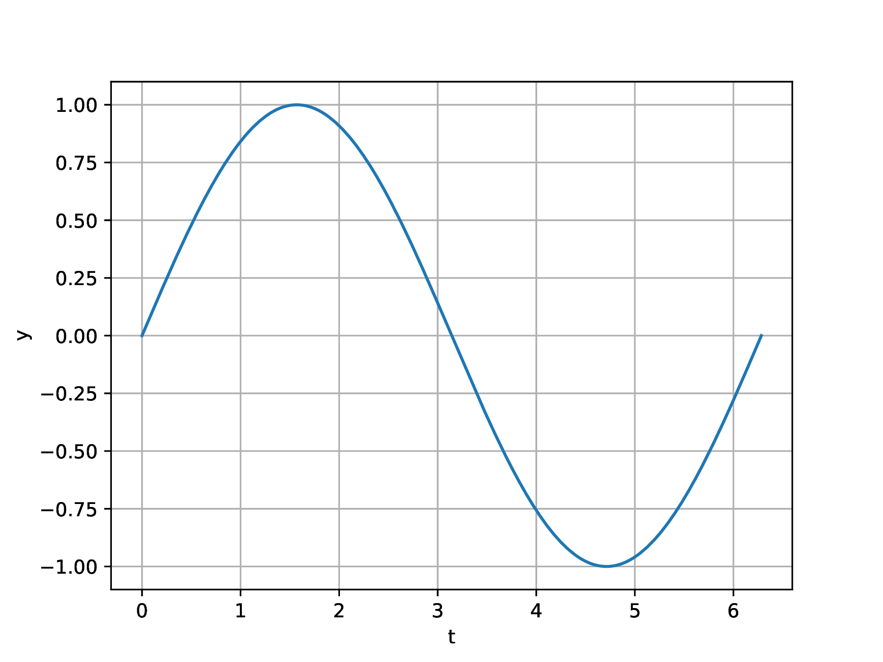
∴	clf(); t=LinRange(0,2*π,180); y=sin.(t);

∴	plot(t,y); grid("on"); xlabel("t"); ylabel("y");

∴	cd(homedir()*"/courses/MATH347DS/images");

∴	savefig("L01Fig01.eps");

∴

Figure 1. Sample plot

3.Matrices

3.1.Forming matrices

The real numbers themselves form the vector space $ℛ_{1} = (ℝ, ℝ, +, \cdot)$ , as does any field of scalars, $𝒮_{1} = (S, S, +, \cdot)$ . Juxtaposition of $m$ real numbers has been seen to define the new vector space $ℛ_{m}$ . This process of juxtaposition can be continued to form additional mathematical objects. A matrix is defined as a juxtaposition of compatible vectors. As an example, consider $n$ vectors $𝒂_{1}, 𝒂_{2}, \dots, 𝒂_{n} \in V$ within some vector space $𝒱 = (V, S, +, \cdot)$ . Form a matrix by placing the vectors into a row,

𝑨 = [\begin{array}{llll} 𝒂_{1} & 𝒂_{2} & \dots & 𝒂_{n} \end{array}] .

(13)

To aid in visual recognition of a matrix, upper-case bold Latin letters will be used to denote matrices. The columns of a matrix will be denoted by the corresponding lower-case bold letter with a subscripted index as in equation (13). Note that the number of columns in a matrix can be different from the number of components in each column, as would be the case for matrix $𝑨$ from equation (13) when choosing vectors from, say, the real space $ℛ_{m}$ , $𝒂_{1}, 𝒂_{2}, \dots, 𝒂_{n} \in ℝ^{m}$ .

A vector is identical to a matrix with a single column vector

𝑨 = [𝒂_{1}] \equiv 𝒂_{1},

and a scalar is identical to a mtrix with a single column vector that has just one component

𝑨 = [a_{11}] \equiv a_{11} .

3.2.Addition, scaling, transposition of matrices

Since matrices are simply juxtaposition of column vectors, the addition and scaling rules for vectors are carried over for matrices $𝑨, 𝑩 \in ℝ^{m \times n}$

𝑨 + 𝑩 = [\begin{array}{llll} 𝒂_{1} & 𝒂_{2} & \dots & 𝒂_{n} \end{array}] + [\begin{array}{llll} 𝒃_{1} & 𝒃_{2} & \dots & 𝒃_{n} \end{array}],

(14)

α 𝑨 = α [\begin{array}{llll} 𝒂_{1} & 𝒂_{2} & \dots & 𝒂_{n} \end{array}] = [\begin{array}{llll} α 𝒂_{1} & α 𝒂_{2} & \dots & α 𝒂_{n} \end{array}] .

(15)

Similarly, the transpose of a matrix turns column vectors into row vectors

𝑨 = [\begin{array}{llll} 𝒂_{1} & 𝒂_{2} & \dots & 𝒂_{n} \end{array}] \in ℝ^{m \times n}, 𝑨^{T} = [\begin{array}{l} 𝒂_{1}^{T} \\ 𝒂_{2}^{T} \\ ⋮ \\ 𝒂_{n}^{T} \end{array}] \in ℝ^{n \times m} .

(16)

In terms of components

𝑨 = [\begin{array}{llll} a_{1, 1} & a_{1, 2} & \dots & a_{1, n} \\ a_{2, 1} & a_{2, 2} & \dots & a_{2, n} \\ ⋮ & ⋮ & ⋱ & ⋮ \\ a_{m, 1} & a_{m, 2} & a_{m, n} \end{array}] \in ℝ^{m \times n}, 𝑨^{T} = [\begin{array}{llll} a_{1, 1} & a_{2, 1} & \dots & a_{m, 1} \\ a_{1, 2} & a_{2, 2} & \dots & a_{m, 2} \\ ⋮ & ⋮ & ⋱ & ⋮ \\ a_{1, n} & a_{2, n} & a_{m, n} \end{array}] \in ℝ^{n \times m} .

It is readily verified that $𝑨 + 𝑩 = 𝑩 + 𝑨$ , $(𝑨 + 𝑩) + 𝑪 = 𝑨 + (𝑩 + 𝑪)$ , ${(𝑨 + 𝑩)}^{T} = 𝑨^{T} + 𝑩^{T}$ .

3.3.Identity matrix

Consider first $ℛ_{1}$ , the vector space of real numbers. A position vector $𝒓 \in ℛ_{1}$ on the real axis is specified by a single scalar component, $𝒓 = [x]$ , $x \in ℝ$ . Read this to mean that the position $𝒓$ is obtained by traveling $x$ units from the origin at position vector $𝟎 = [0]$ . Look closely at what is meant by “unit” in this context. Since $x$ is a scalar, the mathematical expression $𝒓 = 𝟎 + x$ has no meaning, as addition of a vector to a scalar has not been defined. Recall that scalars were introduced to capture the concept of scaling of a vector, so in the context of vector spaces they always appear as multiplying some vector. The correct mathematical description is $𝒓 = 𝟎 + x 𝒆$ , where $𝒆$ is the unit vector $𝒆 = [1]$ . Taking the components leads to $r_{1} = 0_{1} + x e_{1}$ , where $r_{1}, 0_{1}, e_{1}$ are the first (and in this case only) components of the $𝒓, 𝟎, 𝒆$ vectors. Since $r_{1} = x$ , $0_{1} = 0$ , $e_{1} = 1$ , one obtains the identity $x = 0 + x \cdot 1$ .

Now consider $ℛ_{2}$ , the vector space of positions in the plane. Repeating the above train of thought leads to the identification of two direction vectors $𝒆_{1}$ and $𝒆_{2}$

𝒓 = [\begin{array}{l} x \\ y \end{array}] = x [\begin{array}{l} 1 \\ 0 \end{array}] + y [\begin{array}{l} 0 \\ 1 \end{array}] = x 𝒆_{1} + y 𝒆_{2}, 𝒆_{1} = [\begin{array}{l} 1 \\ 0 \end{array}], 𝒆_{2} = [\begin{array}{l} 0 \\ 1 \end{array}] .

∴	x=2; y=4; e1=[1; 0]; e2=[0; 1]; r=xe1+ye2

$[\begin{array}{c} 2 \\ 4 \end{array}]$ (17)

∴

Continuing the procees to $ℛ_{m}$ gives

𝒙 = [\begin{array}{l} x_{1} \\ x_{2} \\ ⋮ \\ x_{m} \end{array}] = x_{1} 𝒆_{1} + x_{2} 𝒆_{2} + \dots + x_{m} 𝒆_{m}, 𝒆_{1} = [\begin{array}{l} 1 \\ 0 \\ ⋮ \\ 0 \\ 0 \end{array}], 𝒆_{2} = [\begin{array}{l} 0 \\ 1 \\ ⋮ \\ 0 \\ 0 \end{array}], \dots, 𝒆_{m} = [\begin{array}{l} 0 \\ 0 \\ ⋮ \\ 0 \\ 1 \end{array}] .

For arbitrary $m$ , the components are now $x_{1}, x_{2}, \dots, x_{m}$ rather than the alphabetically ordered letters common for $m = 2$ or $m = 3$ . It is then consistent with the adopted notation convention to use $𝒙 \in ℛ_{m}$ to denote the position vector whose components are $(x_{1}, \dots, x_{m})$ . The basic idea is the same as in the previous cases: to obtain a position vector scale direction $𝒆_{1}$ by $x_{1}$ , $𝒆_{2}$ by $x_{2}$ ,..., $𝒆_{m}$ by $x_{m}$ , and add the resulting vectors.

Juxtaposition of the vectors $𝒆_{1}, 𝒆_{2}, \dots, 𝒆_{m}$ leads to the formation of a matrix of special utility known as the identity matrix

𝑰 = [\begin{array}{llll} 𝒆_{1} & 𝒆_{2} & \dots & 𝒆_{m} \end{array}] .

The identity matrix is an example of a matrix in which the number of column vectors $n$ is equal to the number of components in each column vector $m = n$ . Such matrices with equal number of columns and rows are said to be square. Due to entrenched practice an exception to the notation convention is made and the identity matrix is denoted by $𝑰$ , but its columns are denoted the indexed bold-face of a different lower-case letter, $𝒆_{1}, \dots, 𝒆_{m}$ . If it becomes necessary to explicitly state the number of columns in $𝑰$ , the notation $𝑰_{m}$ is used to denote the identity matrix with $m$ columns, each with $m$ components.

4.Linear combinations

4.1.Linear combination as a matrix-vector product

The expression

𝒙 = x_{1} 𝒆_{1} + x_{2} 𝒆_{2} + \dots + x_{m} 𝒆_{m}

expresses the idea of scaling vectors within a set and subsequent addition to form a new vector

𝒙

. The matrix

𝑰 = [\begin{array}{llll} 𝒆_{1} & 𝒆_{2} & \dots & 𝒆_{m} \end{array}]

groups these vectors together in a single entity, and the scaling factors are the components of the vector

𝒙

. To bring all these concepts together it is natural to consider the notation

as a generalization of the scalar expression

x = 1 \cdot x

. It is clear what the operation

𝑰 𝒙

should signify: it should capture the vector scaling and subsequent vector addition

x_{1} 𝒆_{1} + x_{2} 𝒆_{2} + \dots + x_{m} 𝒆_{m}

. A specific meaning is now ascribed to

𝑰 𝒙

by identifying two definitions to one another.

Linear combination.

Definition. (Linear Combination) . The linear combination of vectors $𝒂_{1}, 𝒂_{2}, \dots, 𝒂_{n} \in V$ with scalars $x_{1}, x_{2}, \dots, x_{n} \in S$ in vector space $(V, S, +, \cdot)$ is the vector $𝒃 = x_{1} 𝒂_{1} + x_{2} 𝒂_{2} + \dots x_{n} 𝒂_{n} .$

Matrix-vector product.

Definition. (Matrix-Vector Product) . In the vector space $(V, S, +, \cdot)$ , the product of matrix $𝑨 = [\begin{array}{llll} 𝒂_{1} & 𝒂_{2} & \dots & 𝒂_{n} \end{array}]$ composed of columns $𝒂_{1}, 𝒂_{2}, \dots, 𝒂_{n} \in V$ with the vector $𝒙 \in S_{n}$ whose components are scalars $x_{1}, x_{2}, \dots, x_{n} \in S$ is the linear combination $𝒃 = x_{1} 𝒂_{1} + x_{2} 𝒂_{2} + \dots x_{n} 𝒂_{n} = 𝑨 𝒙 \in V .$

4.2.Linear algebra problem examples

Linear combinations in

E_{2}

and can be combined into a matrix

𝑨 = [\begin{array}{ll} 𝒕 & 𝒏 \end{array}]

. The value of the components

(x_{t}, x_{n})

are the scaling factors and can be combined into a vector

𝒙 = {[\begin{array}{ll} x_{t} & x_{n} \end{array}]}^{T}

. The same force must result irrespective of whether its components are given along the Cartesian axes or the inclined plane directions leading to the equality

Interpret equation (18) to state that the vector

𝒃

could be obtained either as a linear combination of

𝑰

𝒃 = 𝑰 𝒃

, or as a linear combination of the columns of

𝑨

𝒃 = 𝑨 𝒙

. Of course the simpler description seems to be

𝑰 𝒃

for which the components are already known. But this is only due to an arbitrary choice made by a human observer to define the force in terms of horizontal and vertical components. The problem itself suggests that the tangential and normal components are more relevant; for instance a friction force would be evaluated as a scaling of the normal force. The components in this more natural reference system are not known, but can be determined by solving the vector equality

𝑨 𝒙 = 𝒃

, known as a linear system of equations. Procedures to carry this out will be studied in more detail later, but Julia provides an instruction for this common problem, the backslash operator, as in x=A\b.

∴	ex=[1; 0]; ey=[0; 1]; b=[0.2; 0.4]; I=[ex ey]; I*b

$[\begin{array}{c} 0.2 \\ 0.4 \end{array}]$ (19)

∴	θ=π/6; c=cos(θ); s=sin(θ); tvec=[c; s]; nvec=[-s; c];

$[\begin{array}{cc} 0.8660254037844387 & - 0.49999999999999994 \\ 0.49999999999999994 & 0.8660254037844387 \end{array}]$ (20)

$[\begin{array}{c} 0.37320508075688774 \\ 0.2464101615137755 \end{array}]$ (21)

∴	x[1]tvec+x[2]nvec

$[\begin{array}{c} 0.2 \\ 0.4 \end{array}]$ (22)

Note from the above calculations how the same vector is obtained by two different linear combinations

The general problem of determining what description is more insightful is a key question arising in linear algebra applications.

4.3.Multiple linear combinations: matrix products

The expression

𝒃 = 𝑨 𝒙

with

𝑨 \in ℝ^{m \times n}

gives

𝒃

as a linear combination of the

n

columns of

𝑨

. It is often the case that multiple linear combinations are sought, say

p

linear combinations

𝒃_{1}, \dots, 𝒃_{p}

of the vectors

𝒂_{1}, 𝒂_{2}, \dots, 𝒂_{n}

with scaling coefficients given by the vectors

𝒙_{1}, \dots, 𝒙_{p}

. Instead of explicitly writing out each linear combination

it is convenient to group all the scaling coefficient vectors into a matrix

𝑿 = [\begin{array}{lll} 𝒙_{1} & \dots & 𝒙_{p} \end{array}] \in ℝ^{n \times p}

, and all the resulting linear combinations into another matrix

𝑩 = [\begin{array}{lll} 𝒃_{1} & \dots & 𝒃_{p} \end{array}] \in ℝ^{m \times p}

, and state that

thus defining matrix-matrix multiplication as the juxtaposition of several matrix-vector multiplications. Note that

𝑨 \in ℝ^{m \times n}

must have as many columns as

𝑿 \in ℝ^{n \times p}

has rows, and the resulting matrix

𝑩 \in ℝ^{m \times p}

has as many rows as

𝑨

and as many columns as

𝑿

The above definition of the matrix products can also be described in terms of components as

5.Vectors and matrices in data science

The above examples highlight some essential aspects of linear algebra in the context of data science applications.

Data science seeks to extract regularity directly from available data, not necessarily invoking any additional hypotheses. The typical scenario is that immense amounts of data are available, with limited capability of human analysis. In this context it is apparent that the least squares problem is of greater interest than solving a linear system with a square matrix. It should also be clear that while computation by hand of small examples is useful to solidify theroretical concepts, it is essential to become proficient in the use of software that can deal with large data sets, such as Julia.

Vectors and Matrices

1.Numbers

1.1.Number sets

1.2.Quantities described by a single number

1.3.Quantities described by multiple numbers

2.Vectors

2.1.Vector spaces

2.2.Real vector space $ℛ_{m}$

Column vectors.

Row vectors.

Compatible vectors.

2.3.Working with vectors

Ranges.

Visualization.

3.Matrices

3.1.Forming matrices

3.2.Addition, scaling, transposition of matrices

3.3.Identity matrix

4.Linear combinations

4.1.Linear combination as a matrix-vector product

Linear combination.

Matrix-vector product.

4.2.Linear algebra problem examples

Linear combinations in $E_{2}$ .

4.3.Multiple linear combinations: matrix products

5.Vectors and matrices in data science

Vectors and Matrices

1.Numbers

1.1.Number sets

1.2.Quantities described by a single number

1.3.Quantities described by multiple numbers

2.Vectors

2.1.Vector spaces

2.2.Real vector space ℛm

Column vectors.

Row vectors.

Compatible vectors.

2.3.Working with vectors

Ranges.

Visualization.

3.Matrices

3.1.Forming matrices

3.2.Addition, scaling, transposition of matrices

3.3.Identity matrix

4.Linear combinations

4.1.Linear combination as a matrix-vector product

Linear combination.

Matrix-vector product.

4.2.Linear algebra problem examples

Linear combinations in E2.

4.3.Multiple linear combinations: matrix products

5.Vectors and matrices in data science

2.2.Real vector space $ℛ_{m}$

Linear combinations in $E_{2}$ .