1.Functions
1.1.Relations
The previous chapter focused on mathematical expression of the concept of quantification, the act of associating human observation with measurements, as a first step of scientific inquiry. Consideration of different types of quantities led to various types of numbers, vectors as groupings of numbers, and matrices as groupings of vectors. Symbols were introduced for these quantities along with some intial rules for manipulating such objects, laying the foundation for an algebra of vectors and matrices. Science seeks to not only observe, but to also explain, which now leads to additional operations for working with vectors and matrices that will define the framework of linear algebra.
Explanations within scientific inquiry are formulated as hypotheses, from which predictions are derived and tested. A widely applied mathematical transcription of this process is to organize hypotheses and predictions as two sets and , and then construct another set of all of the instances in which an element of is associated with an element in . The set of all possible instances of and , is the Cartesian product of with , denoted as , a construct already encountered in the definition of the real 2-space where . Typically, not all possible tuples are relevant leading to the following definition.
The key concept is that of associating an input with an output . Inverting the approach and associating an output to an input is also useful, leading to the definition of an inverse relation as , . Note that an inverse exists for any relation, and the inverse of an inverse is the original relation, . From the above, a relation is a triplet (a tuple with three elements), , that will often be referred to by just its last member .
Homogeneous relations.
1.2.Functions
Functions between sets and are a specific type of relationship that often arise in science. For a given input , theories that predict a single possible output are of particular scientific interest.
The above intuitive definition can be transcribed in precise mathematical terms as is a function if and implies . Since it's a particular kind of relation, a function is a triplet of sets , but with a special, common notation to denote the triplet by , with and the property that . The set is the domain and the set is the codomain of the function . The value from the domain is the argument of the function associated with the function value . The function value is said to be returned by evaluation .
Whereas all relations can be inverted, and inversion of a function defines a new relation, but which might not itself be a function. For example the relation is a function, but its inverse is not.
Familiar functions include:
-
the trigonometric functions , that for argument return the function values giving the Cartesian coordinates of a point on the unit circle at angular extent from the -axis;
-
the exponential and logarithm functions , , as well as power and logarithm functions in some other base ;
-
polynomial functions , defined by a succession of additions and multiplications
Simple functions such as sin, cos, exp, log, are predefined in Julia, and can be applied to each component of a vector argument by broadcasting, denoted by a period in front of the paranteses enclosing the argument.
∴ |
θ=π; [sin(θ) cos(θ) exp(θ) log(θ)] |
(1)
∴ |
θ=0:π/6:π; short(x)=round(x,digits=6); short.(sin.(θ))' |
(2)
∴ |
short.(log2.(1:8))' |
(3)
∴ |
A construct that will be often used is to interpret a vector within as a function, since with components also defines a function , with values . As the number of components grows the function can provide better approximations of some continuous function through the function values at distinct sample points .
The above function examples are all defined on a domain of scalars or naturals and returned scalar values. Within linear algebra the particular interest is on functions defined on sets of vectors from some vector space that return either scalars , or vectors from some other vector space , . The codomain of a vector-valued function might be the same set of vectors as its domain, . The fundamental operation within linear algebra is the linear combination with , . A key aspect is to characterize how a function behaves when given a linear combination as its argument, for instance or
1.3.Linear functionals
Consider first the case of a function defined on a set of vectors that returns a scalar value. These can be interpreted as labels attached to a vector, and are very often encountered in applications from natural phenomena or data analysis.
| (4) |
1.4.Linear mappings
Consider now functions from vector space to another vector space . As before, the action of such functions on linear combinations is of special interest.
| (5) |
The image of a linear combination through a linear mapping is another linear combination , and linear mappings are said to preserve the structure of a vector space.
Note that defined as represents a line in the -plane, but is not a linear mapping for since
Matrix-vector multiplication has been introduced as a concise way to specify a linear combination
with the columns of the matrix, . This is a linear mapping between the real spaces , , , and indeed any linear mapping between real spaces can be given as a matrix-vector product. Consider some
Applying the linear mapping to leads to
The matrix with columns now allows finding
through a matrix-vector multiplication for any input vector . The matrix thus defined is a representation of the linear mapping . As will be shown later, it is not the only possible representation.
2.Measurements
Vectors within the real space can be completely specified by real numbers, and is large in many realistic applications. The task of describing the elements of a vector space by simpler means arises. Within data science this leads to classification problems in accordance with some relevant criteria, and one of the simplest classifications is to attach a scalar label to a vector. Commonly encountered labels include the magnitude of a vector or its orientation with respect to another vector.
2.1.Norms
The above observations lead to the mathematical concept of a norm as a tool to evaluate vector magnitude. Recall that a vector space is specified by two sets and two operations, , and the behavior of a norm with respect to each of these components must be defined. The desired behavior includes the following properties and formal definition.
- Unique value
-
The magnitude of a vector should be a unique scalar, requiring the definition of a function. The scalar could have irrational values and should allow ordering of vectors by size, so the function should be from to , . On the real line the point at coordinate is at distance from the origin, and to mimic this usage the norm of is denoted as , leading to the definition of a function , .
- Null vector case
-
Provision must be made for the only distinguished element of , the null vector . It is natural to associate the null vector with the null scalar element, . A crucial additional property is also imposed namely that the null vector is the only vector whose norm is zero, . From knowledge of a single scalar value, an entire vector can be determined. This property arises at key junctures in linear algebra, notably in providing a link to mathematical analysis, and is needed to establish the fundamental theorem of linear algbera or the singular value decomposition encountered later.
- Scaling
-
Transfer of the scaling operation property leads to imposing . This property ensures commensurability of vectors, meaning that the magnitude of vector can be expressed as a multiple of some standard vector magnitude .
- Vector addition
-
Position vectors from the origin to coordinates on the real line can be added and . If however the position vectors point in different directions, , , then . For a general vector space the analogous property is known as the triangle inequality, for .
-
;
-
;
-
.
A commonly encountered norm of is the Euclidean norm
useful in many physics applications. The form of the above norm, square root of sum of squares of components, can be generalized to obtain other useful norms.
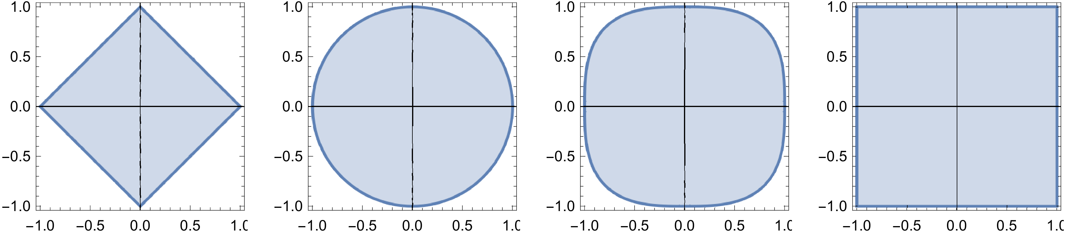
| (6) |
Note that the Euclidean norm corresponds to , and is often called the -norm. Denote by the largest component in absolute value of . As increases, becomes dominant with respect to all other terms in the sum suggesting the definition of an inf-norm by
This also works for vectors with equal components, since the fact that the number of components is finite while can be used as exemplified for , by , with .
Vector norms arise very often in applications, especially in data science since they can be used to classify data, and are implemented in software systems such as Julia in which the norm function with a single argument computes the most commonly encountered norm, the -norm. If a second argument is specified the -norm is computed.
∴ |
x=[1; 1; 1]; [norm(x) sqrt(3)] |
(7)
∴ |
m=9; x=ones(m,1); [norm(x) sqrt(m)] |
(8)
∴ |
m=4; x=ones(m,1); [norm(x,1) m] |
(9)
∴ |
2.2.Inner product
Norms are functionals that define what is meant by the size of a vector, but are not linear. Even in the simplest case of the real line, the linearity relation is not verified for , . Nor do norms characterize the familiar geometric concept of orientation of a vector. A particularly important orientation from Euclidean geometry is orthogonality between two vectors. Another function is required, one that would take two vector arguments to enable characterizing their relative orientation. It would return a scalar, hence , with often chosen as the set of real numbers.
- Symmetry
-
For any , .
- Linearity in second argument
-
For any , , .
- Positive definiteness
-
For any , .
A commonly encountered inner product is the dot product of two vectors
Using the convention of representing as column vectors, the dot product is also expressed as
and is therefore a matrix multiplication between and resulting in a scalar, also referred to as a scalar product. Inner products also provide a procedure to evaluate geometrical quantities and relationships.
- Vector norm
-
The square of the 2-norm of is given as
In general, the square root of satisfies the properties of a norm, and is called the norm induced by an inner product
A real space together with the scalar product and induced norm defines an Euclidean vector space .
- Orientation
-
In the point specified by polar coordinates has the Cartesian coordinates , , and position vector . The inner product
is seen to contain information on the relative orientation of with respect to . In general, the angle between two vectors with any vector space with a scalar product can be defined by
which becomes
in a Euclidean space, .
- Orthogonality
-
In two vectors are orthogonal if the angle between them is such that , and this can be extended to an arbitrary vector space with a scalar product by stating that are orthogonal if . In vectors are orthogonal if .
3.Linear mapping matrices
3.1.Common geometric transformations
Several geometric transformations are linear mappings and are widely used in applications.
Stretching.
The matrix associated with stretching is
and has a remarkably simple form known as a diagonal matrix.
Projection.
The resulting vector is has the same number of components as , and is of length in the direction of , stated as
The matrix associated with projection is
The unit vector is at angle with respect to ,
and the projection of along is
Gathering projections of all the unit vectors within the identity matrix gives
Note that contains column vectors that are all scalings of the vector, by coefficients that are the components of itself. Since scaling is a linear combination, the above linear combinations can be expressed as a matrix-matrix product
leading to the remarkably simple expression
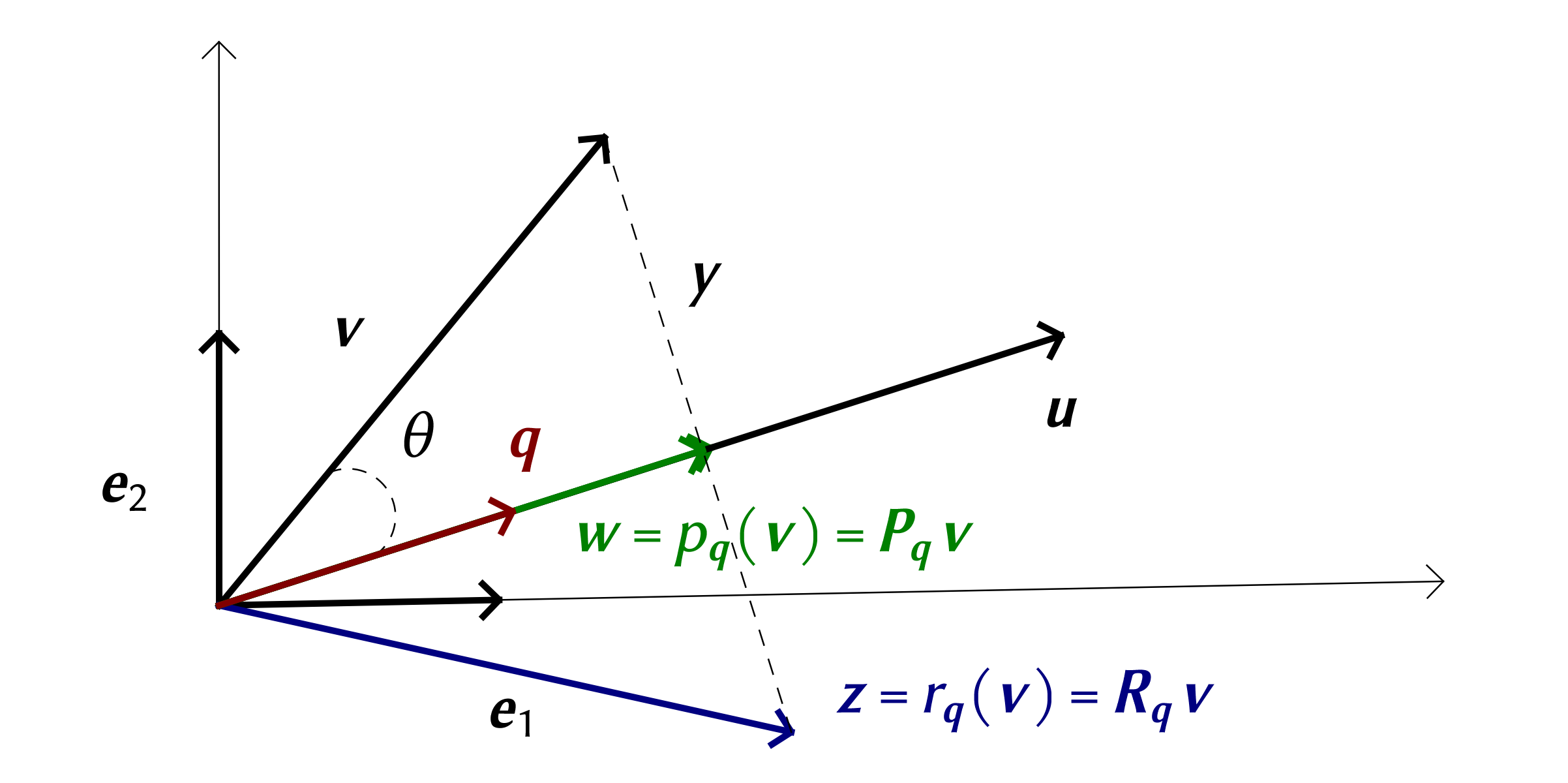
Reflection.
that can be interpreted as stating that the projection is obtained from by addition of the vector . The reflection of across is obtained by starting at , and adding ,
The reflection matrix results
Rotation in .

Rotation in .
3.2.Matrix-matrix product
From two functions and , a composite function, , is defined by
Consider linear mappings between Euclidean spaces , . Recall that linear mappings are expressed as matrix vector multiplications
The composite function is , defined by
Note that the intemediate vector is subsequently multiplied by the matrix . The composite function is itself a linear mapping
so it also can be expressed a matrix-vector multiplication
| (10) |
Using the above, is defined as the product of matrix with matrix
The columns of can be determined from those of by considering the action of on the the column vectors of the identity matrix . First, note that
| (11) |
The above can be repeated for the matrix giving
| (12) |
Combining the above equations leads to , or
From the above the matrix-matrix product is seen to simply be a grouping of all the products of with the column vectors of ,
The above results can readily be verified computationally.
∴ |
a1=[1; 2]; a2=[3; 4]; A=[a1 a2] |
(13)
∴ |
b1=[-1; 1; 3]; b2=[2; -2; 3]; B=[b1 b2] |
(14)
∴ |
C=B*A |
(15)
∴ |
c1=B*a1; c2=B*a2; [c1 c2] |
(16)
∴ |