Vector Space Dimension

Synopsis. The vector subspaces of a matrix characterize what vectors can or cannot be reached by linear combination of matrix columns or rows. How large are these subspaces? An answer is provided by the concept of minimal spanning sets, and the number of vectors in a minimal spanning set allows a precise definition of the intuitive concept of dimension. Upon completion of the framework for vector operations, a first example of the relevance of the theory is considered in the problem of classification of electrocardiograms as indicators of healthy or diseased states.

If $𝑨\in {ℝ}^{m\times n}$ contains $n$ linearly independent vectors ${𝒂}_1,\dots ,{𝒂}_n\in {ℝ}^m$ the nullspace of $𝑨$ only contains one element, the zero vector.

1.2.Orthogonality

Establishing linear independence through the above definition requires algebraic calculations to deduce that $x_1{𝒂}_1+\dots +x_n{𝒂}_n=𝟎$ necessarily implies $x_1=0$, $x_2=0$,…,$x_n=0$. There is an important case suggested by the behavior of the column vectors of the identity matrix $𝑰$ that simplifies the calculations. Distinct column vectors ${𝒆}_1,\dots ,{𝒆}_m$ within $𝑰$ are orthogonal

and each individual vector is of unit 2-norm

In this case multiplying the equation $x_1{𝒆}_1+\dots +x_m{𝒆}_m=𝟎$ by ${𝒆}_j^T$ immediately leads to $x_j=0$, and the column vectors of $𝑰$ are linearly independent. In general any orthogonal set of vectors ${𝒖}_1,\dots ,{𝒖}_n$ are linearly independent by the same argument. In matrix terms, the vectors are collected into a matrix $𝑼=\left[\begin{array}{llll}{𝒖}_1& {𝒖}_2& \dots & {𝒖}_n\end{array}\right]$ and

Definition. The column vectors ${𝒖}_1,{𝒖}_2,\dots ,{𝒖}_n\in {ℝ}^m$ of matrix $𝑼\in {ℝ}^{m\times n}$ are orthogonal if

An especially simple and useful case is when the norms of all orthogonal vectors are equal to one.

Definition. The column vectors ${𝒒}_1,{𝒒}_2,\dots ,{𝒒}_n\in {ℝ}^m$ of matrix $𝑸\in {ℝ}^{m\times n}$ are orthonormal if

Somewhat confusingly a square matrix with orthonormal columns is said to be orthogonal.

Definition. The matrix $𝑸\in {ℝ}^{m\times m}$ is orthogonal if

Example. The rotation matrix in ${ℝ}^2$ is orthogonal,

Example. A rotation matrix in ${ℝ}^3$ is orthogonal,

Example. The reflection matrix across direction $𝒒$ of unit norm in ${ℝ}^m$

is orthogonal

since $𝒒{𝒒}^T𝒒{𝒒}^T=𝒒\left({𝒒}^T𝒒\right){𝒒}^T=𝒒\left(1\right){𝒒}^T=𝒒{𝒒}^T$.

2.Basis and dimension

2.1.Minimal spanning sets

Vector spaces are closed under linear combination, and the span of a vector set $ℬ=\{{𝒂}_1,{𝒂}_2,\dots \}$ defines a vector subspace. If the entire set of vectors can be obtained by a spanning set, $V=\mathrm{span}ℬ$, extending $ℬ$ by an additional element $𝒞=ℬ\cup \left\{𝒃\right\}$ would be redundant since $\mathrm{span}ℬ=\mathrm{span}𝒞$. Avoinding redundancy leads to a consideration of a minimal spanning set. This is formalized by the concept of a basis, and also allows leads to a characterization of the size of a vector space by the cardinality of a basis set.

Definition. A set of vectors ${𝒖}_1,\dots ,{𝒖}_n\in U$ is a basis for vector space $𝒰=(U,S,+,\cdot )$ if

Definition. The number $n$ of vectors ${𝒖}_1,\dots ,{𝒖}_n\in U$ within a basis is the dimension of the vector space $𝒰=(U,S,+,\cdot )$.

The above definitions underlie statements such as “${ℝ}^3$ represents three-dimensional space”. Since any $𝒗\in {ℝ}^3$ can be expressed as

it results that $\{{𝒆}_1,{𝒆}_2,{𝒆}_3\}$ is a spanning set. The equation $x_1{𝒆}_1+x_2{𝒆}_2+x_3{𝒆}_3=𝟎$ leads to

hence $\{{𝒆}_1,{𝒆}_2,{𝒆}_3\}$ are independent, and therefore form a basis. The cardinality of the set $\{{𝒆}_1,{𝒆}_2,{𝒆}_3\}$ is equal to three, and, indeed, ${ℝ}^3$ represents three-dimensional space.

2.2.Dimensions of matrix spaces

The domain ${ℝ}^n$ and co-domain ${ℝ}^m$ of the linear mapping $𝒇:{ℝ}^n\to {ℝ}^m$, $𝒇\left(𝒙\right)=𝑨𝒙$, are vector spaces. Within these vector spaces, subspaces associated with the linear mapping are defined by:

• $C\left(𝑨\right)$ the column space of $𝑨$, $C\left(𝑨\right)\le {ℝ}^m$

• $C\left({𝑨}^T\right)$ the row space of $𝑨$, $C\left({𝑨}^T\right)\le {ℝ}^n$

• $N\left(𝑨\right)$ the null space of $𝑨$, $N\left(𝑨\right)\le {ℝ}^n$

• $N\left({𝑨}^T\right)$ the left null space of $𝑨$, or null space of ${𝑨}^T$, $N\left({𝑨}^T\right)\le {ℝ}^m$.

The dimensions of these subspaces arise so often in applications to warrant formal definition.

Definition. The rank of a matrix $𝑨\in {ℝ}^{m\times n}$ is the dimension of its column space.

Definition. The nullity of a matrix $𝑨\in {ℝ}^{m\times n}$ is the dimension of its null space.

The dimension of the row space is equal to that of the column space. This is a simple consequence of how scalars are organized into vectors. When the preferred organization is into column vectors, a linear combination is expressed as

The same linear combination can also be expressed through rows by taking the transpose, an operation that swaps rows and columns,

Any statment about the linear combination of column vectors $x_1{𝒂}_1+\cdots +x_n{𝒂}_n$ also holds for the linear combination of row vectors $x_1{𝒂}_1^T+\cdots +x_n{𝒂}_n^T$. In particular the dimension of the column space equals that of the row space.

3.Signal compression

3.1.Electrocardiograms

The first forays of the significance of matrix-associated subspaces through geometry of lines or planes is useful, but belie the utility of these concepts in applications. Consider the problem of long-term care for cardiac patients. Electrocardiograms (ECGs) are recorded periodically, often over decades and need to be stored for comparison and assessment of disease progression. Heartbeats arise from electrical signals occuring at frequencies of around $f=250$ Hz (cycles/second). A “single-lead” ECG to detect heart arrhythmia can require $T=180$ s recording time, so a vector representation would require $m=fT=4.5\times {10}^4\cong 𝒪\left({10}^5\right)$ components, $𝒃\in {ℝ}^m$,

where component $b_j$ is the voltage recorded at time $t_j=j\left(\delta t\right)$, and $\delta t=1/f$ is the sampling time interval.

The linear combination (4) seems a natural way to organize recorded data, but is it the most insightful? Recall the inclined plane example in which forces seemed to be naturally described in a Cartesian system consisting of the horizontal and vertical directions, yet a more insightful description was seen to correspond to normal and tangential directions. Might there be an alternative linear combination, say

that would represent the ECG in a more meaningful manner? The vectors entering into the linear combination are, as usual, organized into a matrix

such that the ECG is obtained through a matrix-vector product $𝒃=𝑯𝒙,𝒙\in {ℝ}^m$. In particular, in this alternative description, could a smaller number of components suffice for capturing the essence of the ECG? Select the first $n$ components by defining

The two-norm of the vectors' difference is the error $\epsilon ={||𝒃-𝒄||}_2$ incurred by keeping only $n$ components. If $𝒄$ is close to $𝒃$ then $\epsilon$ should be small, and if $n$ is much smaller than $m$, a compressed version of the ECG is obtained.

At first sight, the representations (5,6) might seem more costly than (4) since not only do the scaling factors $𝒙\in {ℝ}^m$ or $𝒚\in {ℝ}^n$ have to be stored, but also the $m^2$ components of $𝑯$ also. This difficulty is eliminated if $𝑯=\left[\begin{array}{llll}{𝒉}_1& {𝒉}_2& \dots & {𝒉}_m\end{array}\right]$ is obtained by some simple rule, much as $𝑰=\left[\begin{array}{llll}{𝒆}_1& {𝒆}_2& \dots & {𝒆}_m\end{array}\right]$ can be specified by any one of a number of procedures.

3.2.The identity matrix revisited

Within the algebraic structure of a vector space there is an identity element $1\in ℝ$ with respect to the operation of scaling the vector $𝒃\in {ℝ}^m$,

Analogously, the identity matrix $𝑰\in {ℝ}^{m\times m}$ acts as an identity element with respect to matrix vector multiplication

Since matrix-matrix multiplication is simply successive matrix-vector multiplications,

the identity matrix $𝑰$ is an identity element for matrix multiplication

Computer storage of the identity matrix $𝑰\in {ℝ}^{m\times m}$ might naively seem to require $m^2$ locations, one for every component, but its remarkable structure implies specification only of a single number, $m$ the size of $𝑰$. The identity matrix can then be reconstructed as needed through a variety of procedures.

Predefined identity operator

In Julia I is a predefined operator from which the full identity matrix can be reconstructed if needed

∴	m=3; Matrix(1.0I,m,m)

${\displaystyle \left[\begin{array}{ccc}1.0& 0.0& 0.0\\ 0.0& 1.0& 0.0\\ 0.0& 0.0& 1.0\end{array}\right]}$

(7)

Component definition

In terms of components

${\displaystyle 𝑰=\left[{\delta }_{ij}\right],1⩽i,j⩽m,{\delta }_{ij}=\{\begin{array}{ll}1& \mathrm{if}i=j\\ 0& \mathrm{otherwise}\end{array}.,}$

where ${\delta }_{ij}$ is known as Kronecker-delta and is readily transcribed in Julia.

∴	δ(i,j) = if i==j return 1 else return 0 end;

∴	Id(m) = [δ(i,j) for i in 1:m, j=1:m]; Id(3)

${\displaystyle \left[\begin{array}{ccc}1& 0& 0\\ 0& 1& 0\\ 0& 0& 1\end{array}\right]}$

(8)

∴

Column vector definition

Another construction is by circular shifts of the column vector ${𝒆}_1={\left[\begin{array}{llll}1& 0& \dots & 0\end{array}\right]}^T\in {ℝ}^m$.

∴	e1T(m) = [1; zeros(m-1,1)]; e1T(3)

${\displaystyle \left[\begin{array}{c}1.0\\ 0.0\\ 0.0\end{array}\right]}$

(9)

∴	ekT(m,k) = circshift(e1T(m),k); [ekT(3,0) ekT(3,1) ekT(3,2)]

${\displaystyle \left[\begin{array}{ccc}1.0& 0.0& 0.0\\ 0.0& 1.0& 0.0\\ 0.0& 0.0& 1.0\end{array}\right]}$

(10)

Diagonal matrix construction

The diagonal structure of $𝑰$ also defines a reconstruction.

∴	Diagonal(ones(3,3))

${\displaystyle \left[\begin{array}{ccc}1.0& 0.0& 0.0\\ 0.0& 1.0& 0.0\\ 0.0& 0.0& 1.0\end{array}\right]}$

(11)

∴

3.3.

Exterior product construction of $𝑰$

A conceptually different reconstruction of $𝑰$ when $m=2^p$ uses block matrix operations and builds up larger matrices from smaller ones. This technique is quite instructive in that it:

• introduces the concept of an outer product that can be compared to inner products;

• introduces the concept of recursive definition.

Since larger versions of the identity matrix will be obtained from smaller ones, a notation to specify the matrix size is needed. Let ${𝑰}_k$ denote the identity matrix of size $m\times m$ with $m=2^k$. Start from $p=0$, $m=1$ in which case ${𝑰}_0=\left[1\right]$, also define

The next matrix in this sequence would be ${𝑰}_2$ in which a block structure can be identified

The scaling coefficients applied to each ${𝑰}_1$ block are recognized to be ${𝑰}_1$ itself. This suggest that the next matrix in the sequence could be obtained as

It is useful to introduce a notation for these operations: ${𝑰}_2={𝑰}_1\otimes {𝑰}_1,{𝑰}_3={𝑰}_1\otimes {𝑰}_2$.

Definition. The exterior product of matrices $𝑨=\left[a_{ij}\right]\in {ℝ}^{m\times n}$ and $𝑩\in {ℝ}^{p\times q}$ is the matrix $𝑪\in {ℝ}^{(mp)\times (nq)}$

Recall that the inner product of $𝒖,𝒗\in {ℝ}^m$ is the scalar ${𝒖}^T𝒗$, and one can think of an inner product as “reducing the dimensions of its factors”. In contrast the exterior product “increases the dimensions of its factors”. An example of the exterior product has already been met, namely the projection matrix along direction $𝒒$ of unit norm ($||𝒒||=1$)

Using the exterior product definition the matrix ${𝑰}_q$ is defined in terms of previous terms in the sequence as

Such definitions based upon previous terms are said to be recursive.

3.4.Walsh-Hadamard matrices

An alternative to specifying the signal $𝒃\in {ℝ}^m$ as the linear combination $𝒃=𝑰𝒃$ is now constructed by a different recursion procedure. As in the identity matrix case let $m=2^p$ and start from $p=0$, $m=1$ with ${𝑯}_0=\left[1\right]$. For the next term choose however

and define in general

Julia can be extended to include definitions of the above Hadamard matrices.

∴ 

using Hadamard

∴ 

H0=hadamard(2^0)

∴ 

H1=hadamard(2^1)

∴ 

H2=hadamard(2^2)

∴ 

The column vectors of the identity matrix are mutually orthogonal as expressed by

The Hadamard matrices have similar behavior in that

and thus be seen to have orthogonal columns.

∴ 

H2'*H2

∴ 

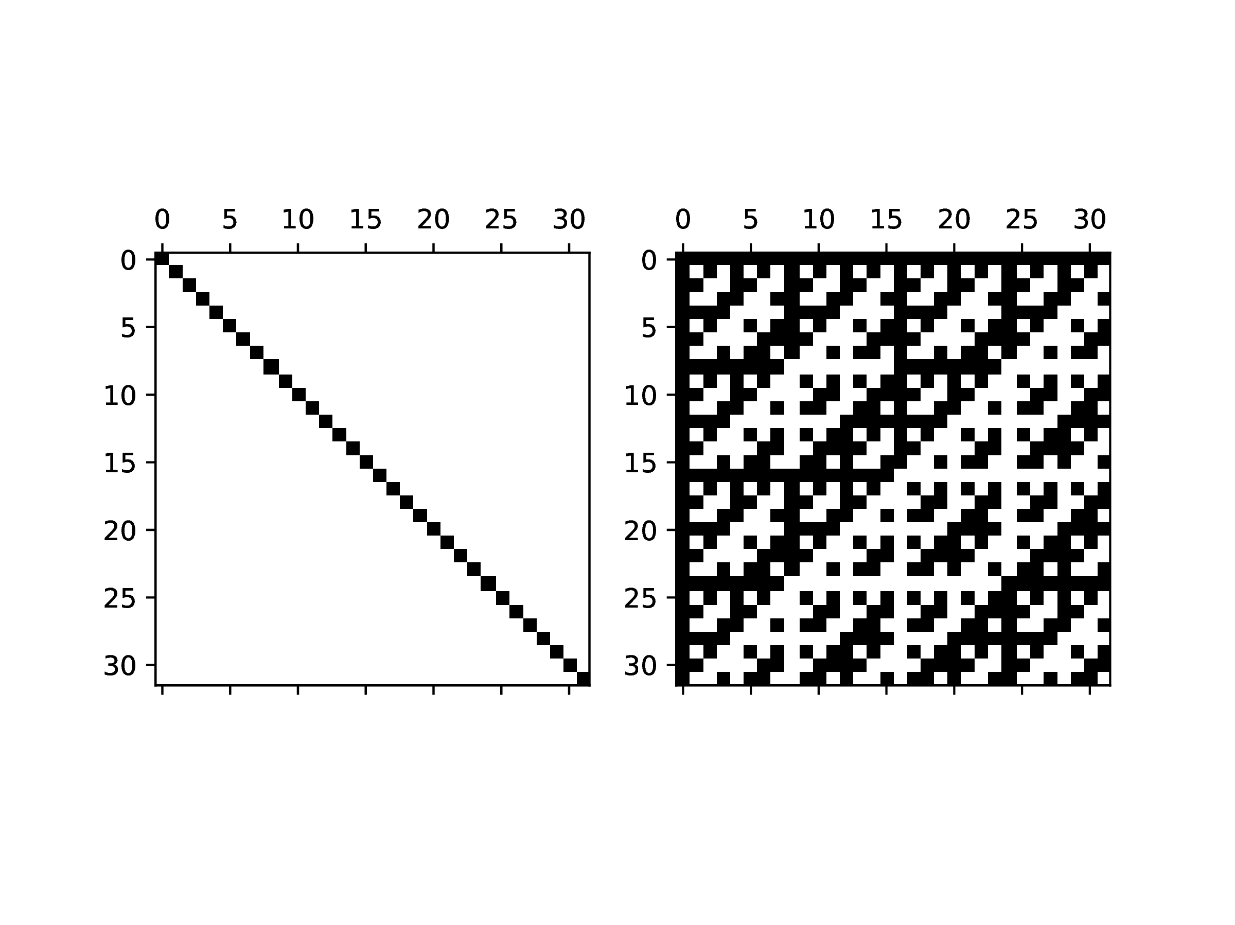
The structure of Hadamard matrices allows a reconstruction from small cases just as simple as that of the identity matrix, but the components of a Hadamard matrix are quite different. Rather than display of the components a graphical visualization is insightful. The spy(A) function displays a plot of the non-zero components of a matrix

∴ 

q=5; m=2^q; Iq=Matrix(1.0I,m,m); Hq=hadamard(m);

∴ 

clf(); subplot(1,2,1); spy(Iq); subplot(1,2,2); spy(Hq.+1);

∴ 

cd(homedir()*"/courses/MATH347DS/images"); savefig("L03Fig01.eps");

∴ 

Figure 1. The structure of the identity and Hadamard matrices for $m=2^5=32$.

3.5.Sample sets and reconstructions

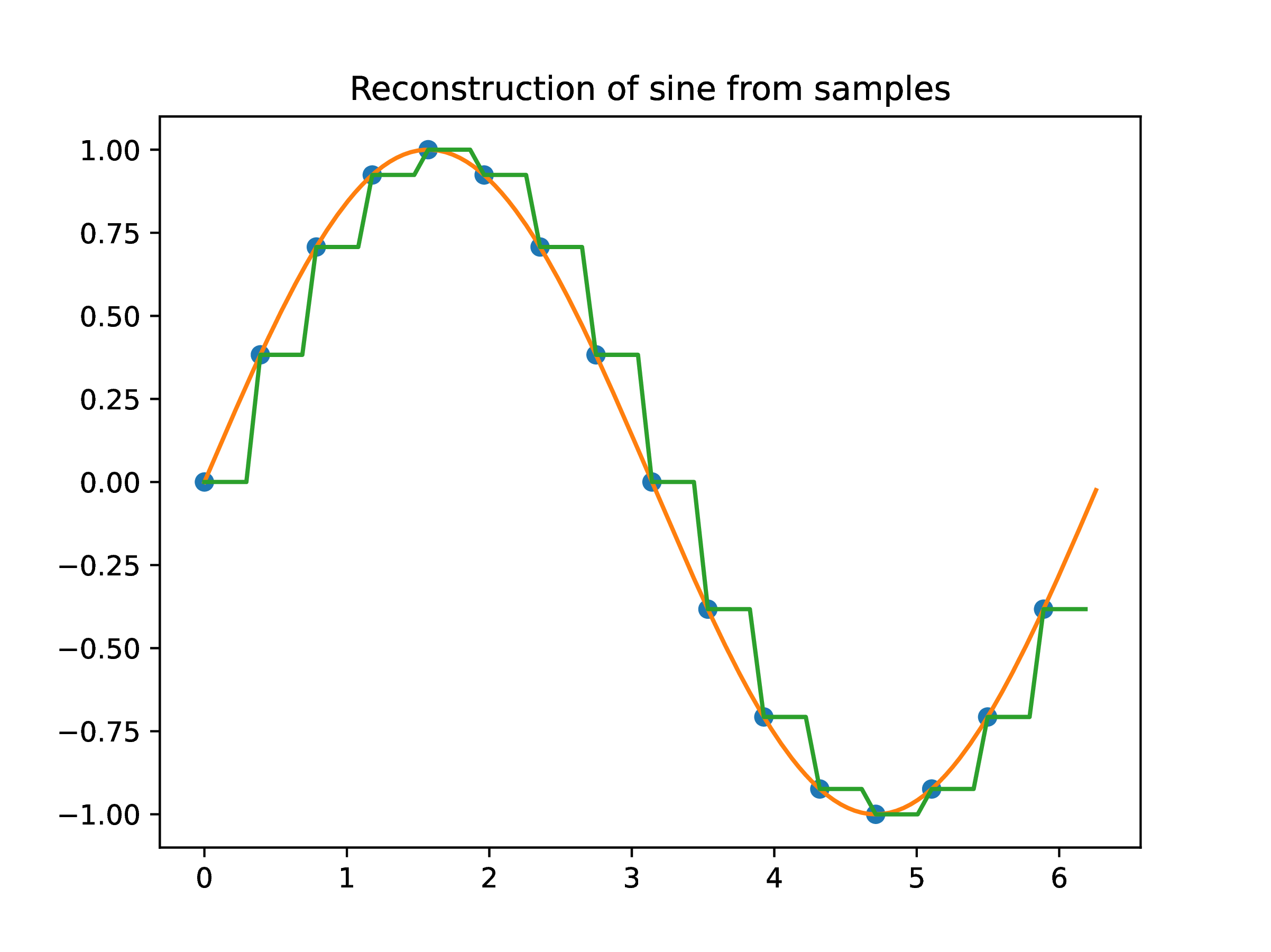
The behavior of the column vectors of $𝑰$ and $𝑯$ is instructive. Denote by $b:ℝ\to ℝ$ the ECG recording that would be obtained measurements were carried out for all $t\in [0,T]$. This is obviously impossible since it would require an infinite number of measurements. In practice, only the values $b_i=b\left(t_i\right)$ are recorded for $t_i=i\left(\delta t\right)$, which is a sample of the infinite set of the possible values. The sample set values are organized into the vector $𝒃$. Function values $b\left(t\right)$ for $t\ne t_i$ can be reconstructed through some assumption, for instance that

The above states that $b\left(t\right)$ remains constant from $t_i$ to $t_i+\delta t$. A simple example when $b\left(t\right)=\sin \left(t\right)$ illustrates the approach.

∴ 

T=2*pi; n=16; δt=T/n; t=(0:n-1)*δt; b=sin.(t);

∴ 

m=n^2; δts=T/m; ts=(0:m-1)*δts; s=sin.(ts);

∴ 

p=4*n; δtw=T/p; tw=(0:p-1)*δtw; w=reshape((b.*[1 1 1 1])',(1,p))';

∴ 

figure(3); clf(); plot(t,b,"o",ts,s,tw,w);

∴ 

title("Reconstruction of sine from samples");

∴ 

savefig("L04Fig02.eps");

∴ 

Figure 2. The reconstruction is a step function.

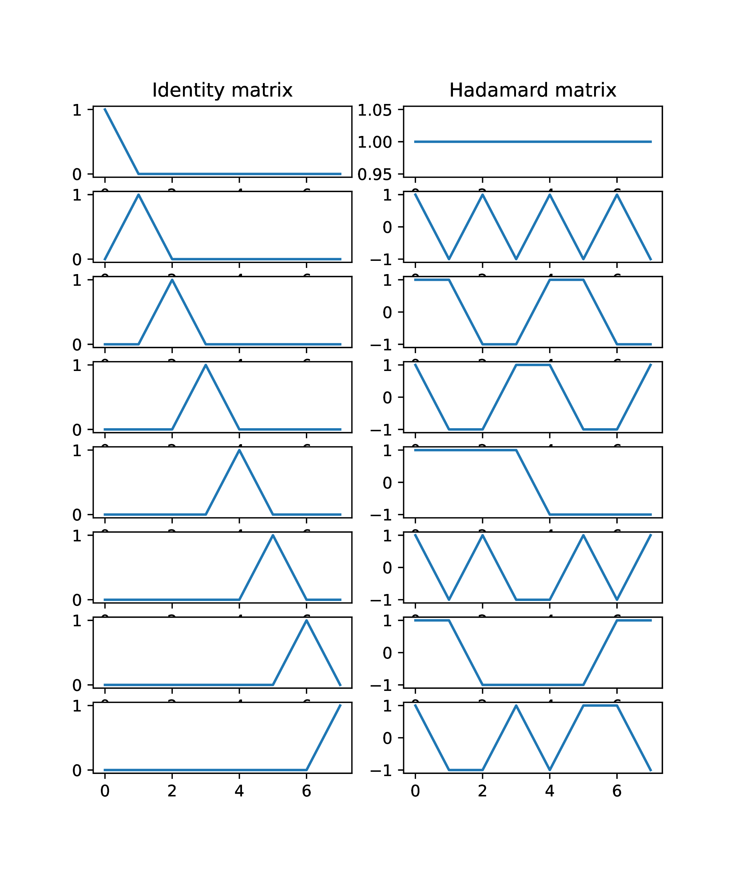
The reconstruction exhibits steps at which the function value changes. The column vectors of $𝑰$ are well suited for such reconstructions.

∴ 

n=8; In=Matrix(1.0I,n,n); Hn=hadamard(n);

∴ 

figure(5); clf();

∴ 

for j=1:n
   subplot(8,2,2*j-1); plot(In[:,j])
   subplot(8,2,2*j);   plot(Hn[:,j])
end

∴ 

title("Column vectors of I");

∴ 

subplot(2,1,2);

∴ 

for j=1:n
   plot(Hn[:,j])
end

∴ 

subplot(8,2,1); title("Identity matrix");

∴ 

subplot(8,2,2); title("Hadamard matrix");

∴ 

savefig("L04Fig03.eps");

∴ 

Figure 3. Comparison of column vectors of $𝑰,𝑯$.

3.6.Naive ECG compression

ECG compression.

are truncated? The scaling coefficients of the Hadamard linear combination are readily found

Consider $𝒖$ to be the truncation of $𝒃=𝑰𝒃$ to $n<m$ terms

Due to the choice of the significance of the components $b_i$ the above simply drops ECG recording times for $t>n\left(\delta t\right)$. The truncation of the Hadamard linear combination

behaves quite differently.

∴ 

using MAT

∴ 

DataFileName = homedir()*"/courses/MATH347DS/data/ecg/ECGData.mat";

∴ 

DataFile = matopen(DataFileName,"r");

∴ 

dict = read(DataFile,"ECGData");

∴ 

data = dict["Data"]';

∴ 

size(data)

∴ 

q=12; m=2^q; k=15; b=data[1:m,k];

∴ 

Iq=Matrix(1.0I,m,m); Hq=hadamard(m); c=(1/m)*transpose(Hq)*b;

∴ 

n=2^10; u=Iq[:,1:n]*b[1:n]; v=Hq[:,1:n]*c[1:n];

∴ 

figure(1); clf(); subplot(3,1,1); plot(b);

∴ 

subplot(3,1,2); plot(u);

∴ 

subplot(3,1,3); plot(v);

∴ 

cd(homedir()*"/courses/MATH347DS/images"); savefig("L03Fig02.eps");

∴ 

Figure 4. Comparison of original ECG (top) containing $m=2^{12}=4096$ time samples with truncated linear combinations based upon $n=2^{10}=1024$ terms of the linear combinations using identity matrix $𝑰$ (middle), and Hadamard matrix $𝑯$ (bottom).

3.7.Basis subsets and compression

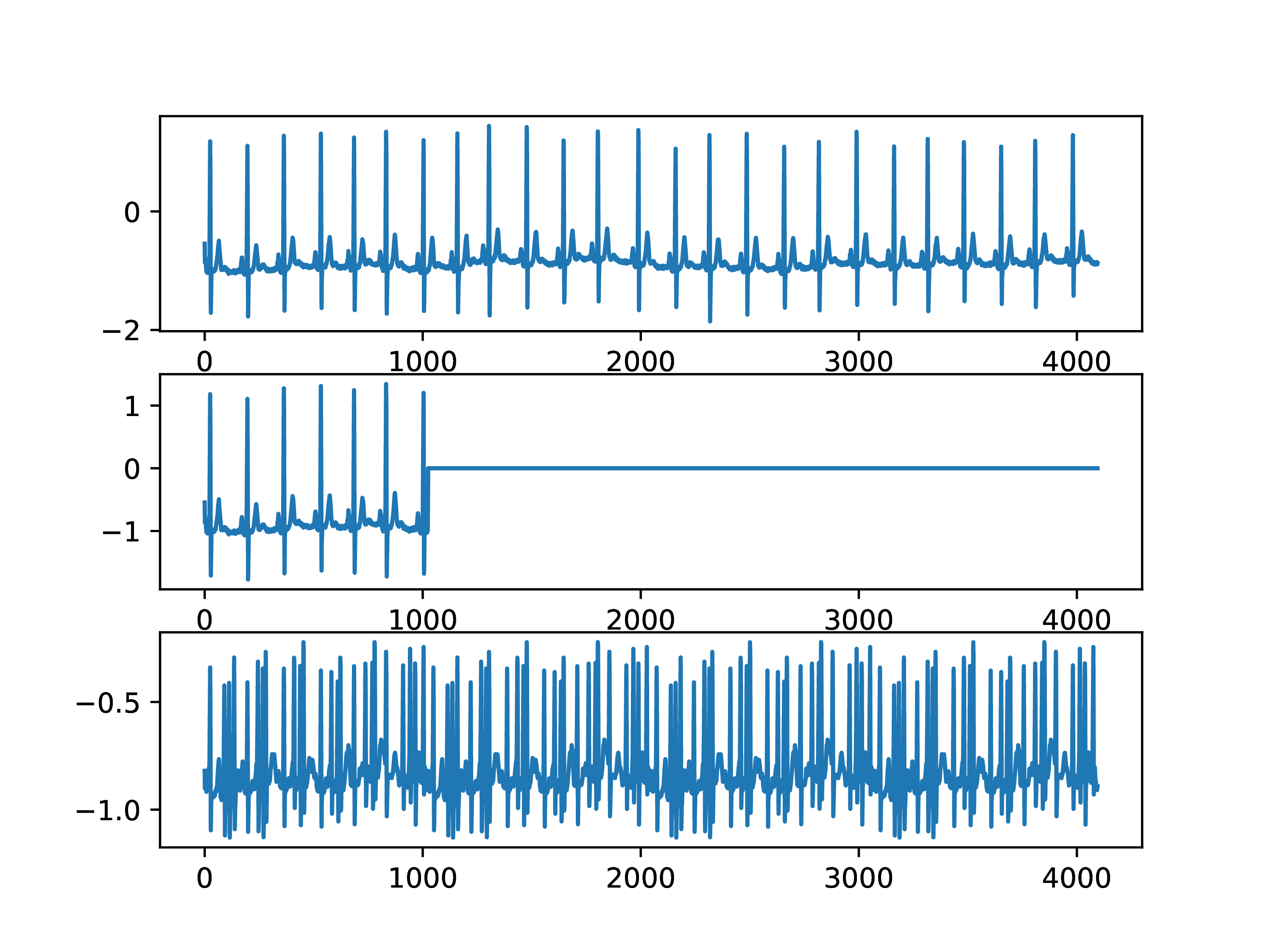Neither of the truncated linear combinations seems particularly useful. Truncation of the $𝑰$-based linear combination cuts off part of the signal, while that of the $𝑯$-based linear combination introduces heart pulses not present in the original signal. The problem is the significance given to the ordering of the vectors into the linear combination. Consider first truncation of $𝒃=𝑰𝒃$ to obtain $𝒖$. Rather than cutting off part of the signal, an alternative data compression is to use a larger time sample, say 4$\delta t$ instead of $\delta t$, a process known as down-sampling,

∴ 

w=fwht(b);

∴ 

figure(6); clf(); plot(c,".");

∴ 

plot(w,".");

∴