Least Squares Approximation

Synopsis. Having established the key theoretical results, the main linear algebra problems can now be solved. The typical scenario within data science applications is that a large dimensional vector representation of some object is available and greater insight is sought by seeking a description in terms of linear combination of a small number of vectors. The large dimensional object might not be exactly recovered and the focus is on obtaining the best possible approximation. In Euclidean spaces with distances measured by the 2-norm, best approximants are readily found by the generalization of the Pythagorean theorem to high-dimensional spaces.

1.Orthogonal projection

Consider a partition of a vector space $U$ into orthogonal subspaces $U=V\oplus W$, $V=W^{\perp }$, $W=V^{\perp }$, typically $U={ℝ}^m$, $V\subset {ℝ}^m$, $W\subset {ℝ}^m$, $\dim V=n$, $\dim W=m-n$. If $𝑽=\left[\begin{array}{ccc}{𝒗}_1& \dots & {𝒗}_n\end{array}\right]\in {ℝ}^{m\times n}$ is a basis for $V$ and $𝑾=\left[\begin{array}{ccc}{𝒘}_1& \dots & {𝒘}_{m-n}\end{array}\right]\in {ℝ}^{m\times (m-n)}$ is a basis for W, then $𝑼=\left[\begin{array}{cccccc}{𝒗}_1& \dots & {𝒗}_n& {𝒘}_1& \dots & {𝒘}_{m-n}\end{array}\right]$ is a basis for $U$. Even though the matrices $𝑽,𝑾$ are not necessarily square, they are said to be orthonormal when all columns are of unit norm and orthogonal to one another. In this case computation of the matrix product ${𝑽}^T𝑽$ leads to the formation of the identity matrix within ${ℝ}^n$

Similarly, ${𝑾}^T𝑾={𝑰}_{m-n}$. Whereas for the square orthogonal matrix $𝑼$ multiplication both on the left and the right by its transpose leads to the formation of the identity matrix

the same operations applied to rectangular orthogonal matrices lead to different results

A simple example is provided by taking $𝑽={𝑰}_{m,n}$, the first $n$ columns of the identity matrix in which case

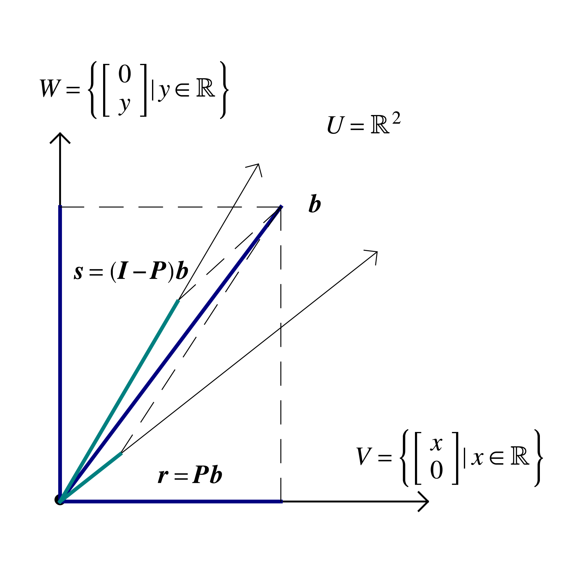
Applying $𝑷=𝑽{𝑽}^T$ to some vector $𝒃\in {ℝ}^m$ leads to a vector $𝒓=𝑷𝒃$ whose first $n$ components are those of $𝒃$, and the remaining $m-n$ are zero. The subtraction $𝒃-𝒓$ leads to a new vector $𝒔=(𝑰-𝑷)𝒃$ that has the first components equal to zero, and the remaining $m-n$ the same as those of $𝒃$. Such operations are referred to as projections, and for $𝑽={𝑰}_{m,n}$ correspond to projection onto the span$\{{𝒆}_1,\dots ,{𝒆}_n\}$.

Returning to the general case, the orthogonal matrices $𝑼\in {ℝ}^{m\times m}$, $𝑽\in {ℝ}^{m\times n}$, $𝑾\in {ℝ}^{m\times (m-n)}$ are associated with linear mappings $𝒃=𝒇\left(𝒙\right)=𝑼𝒙$, $𝒓=𝒈\left(𝒃\right)=𝑷𝒃$, $𝒔=𝒉\left(𝒃\right)=(𝑰-𝑷)𝒃$. The mapping $𝒇$ gives the components in the $𝑰$ basis of a vector whose components in the $𝑼$ basis are $𝒙$. The mappings $𝒈,𝒉$ project a vector onto span$\{{𝒗}_1,\dots ,{𝒗}_n\}$, span$\{{𝒘}_1,\dots ,{𝒘}_{m-n}\}$, respectively. When $𝑽,𝑾$ are orthogonal matrices the projections are also orthogonal $𝒓\perp 𝒔$. Projection can also be carried out onto nonorthogonal spanning sets, but the process is fraught with possible error, especially when the angle between basis vectors is small, and will be avoided henceforth. Notice that projection of a vector already in the spanning set simply returns the same vector, which leads to a general definition.

Definition. The mapping is called a projection if $𝒇\circ 𝒇=𝒇$, or if for any $𝒖\in U$, $𝒇\left(𝒇\left(𝒖\right)\right)=𝒇\left(𝒖\right)$. With $𝑷$ the matrix associated $𝒇$, a projection matrix satisfies ${𝑷}^2=𝑷$.

Orthogonal projections onto the column space $C\left(𝑸\right)$ of an orthonormal matrix are of great practical utility, and satisfy the above definition

2.Gram-Schmidt algorithm

Orthonormal vector sets $\{{𝒒}_1,\dots ,{𝒒}_n\}$ are of the greatest practical utility, leading to the question of whether some such a set can be obtained from an arbitrary set of vectors $\{{𝒂}_1,\dots ,{𝒂}_n\}$. This is possible for independent vectors, through what is known as the Gram-Schmidt algorithm

1. Start with an arbitrary direction ${𝒂}_1$

2. Divide by its norm to obtain a unit-norm vector ${𝒒}_1={𝒂}_1/||{𝒂}_1||$

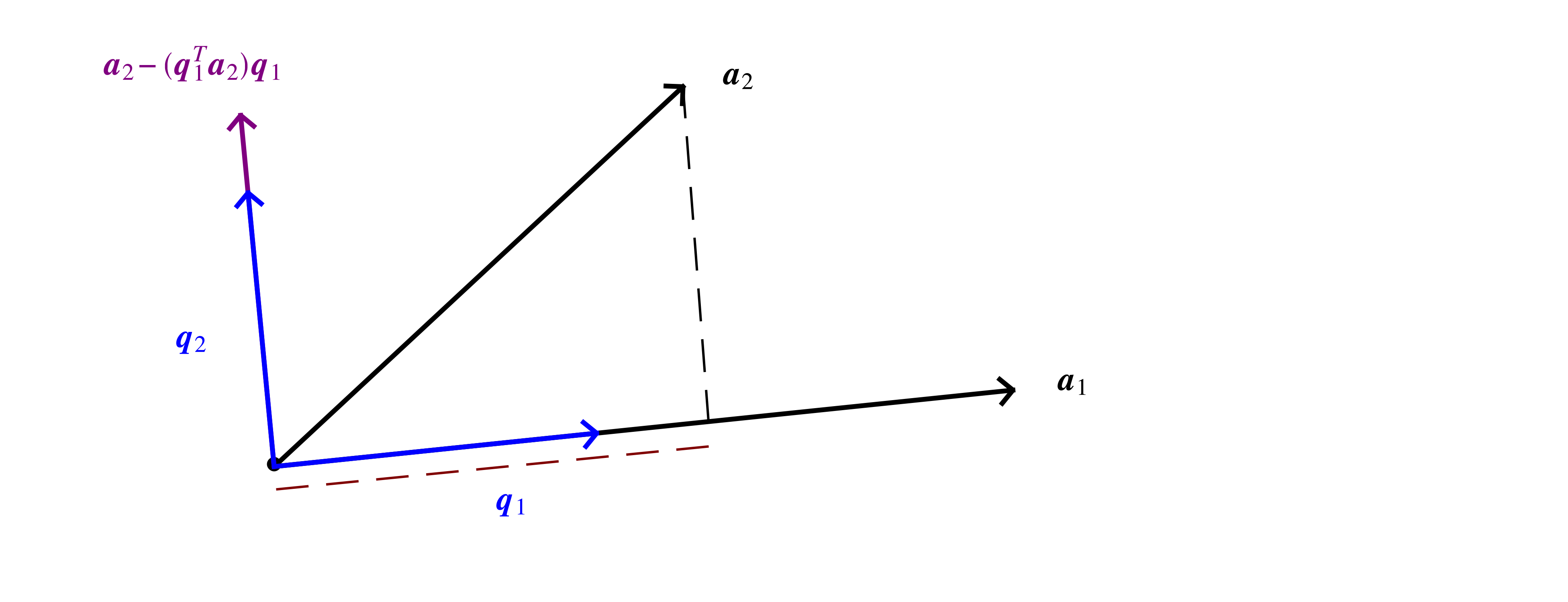
3. Choose another direction ${𝒂}_2$

4. Subtract off its component along previous direction(s) ${𝒂}_2-\left({𝒒}_1^T{𝒂}_2\right){𝒒}_1$

5. Divide by norm ${𝒒}_2=({𝒂}_2-\left({𝒒}_1^T{𝒂}_2\right){𝒒}_1)/||{𝒂}_2-\left({𝒒}_1^T{𝒂}_2\right){𝒒}_1||$

6. Repeat the above

The above geometrical description can be expressed in terms of matrix operations as

equivalent to the system

The system is easily solved by forward substitution resulting in what is known as the (modified) Gram-Schmidt algorithm, transcribed below both in pseudo-code and in Julia.

∴ 

function mgs(A)
  m,n=size(A); Q=A; R=eye(n);
  for i=1:n
    R[i,i] = sqrt(Q[:,i]'*Q[:,i]);
    if (R[i,i]<eps) break;
    Q[:,i] = Q[:,i]/R[i,i];
    for j=i+1:n
      R[i,j] = Q[:,i]'*A[:,j];
      Q[:,j] = Q[:,j] - R[i,j]*Q[:,i];
    end;
  end;
  return Q,R
end

The input matrix $𝑨$ might have linearly dependent columns in which case $r_{ii}\approx 0$ for some $i$, and the if-instruction interrupts the algorithm. The Gram-Schmidt algorithm furnishes a factorization

with $𝑸\in {ℝ}^{m\times n}$ an orthonormal matrix and $𝑹\in {ℝ}^{n\times n}$ an upper triangular matrix, known as the $QR$-factorization. Since the column vectors within $𝑸$ were obtained through linear combinations of the column vectors of $𝑨$, $C\left(𝑨\right)=C\left(𝑸\right)$. The $QR$-factorization is of great utility in solving problems within linear algebra.

3.Least squares problems in ${ℝ}^m$

3.1.Problem formulation and solution by orthogonal projection

A typical situation in applications is that a vector $𝒚\in {ℝ}^m$ represents a complex object with $m\gg 1$. A simpler representation of the object is sought through a linear combination $𝒗=𝑨𝒄$, with $𝑨\in {ℝ}^{m\times n}$ and $n<m$, usually $m\ll n$ (Fig. 1).

Figure 1. Least squares problem: find $𝒗\in C\left(𝑨\right)$, $𝑨\in {ℝ}^{m\times n}$ closest to some given $𝒚$ in the 2-norm

The magnitude of the difference between the exact object $𝒚$ and the approximation $𝑨𝒄$ is measured through a norm, and in least squares the 2-norm is adopted. The problem is to minimize the error $\epsilon =||𝒆||=||𝒚-𝑨𝒄||={\left({𝒆}^T𝒆\right)}^{1/2}$. This is stated mathematically as

${\displaystyle {min}_{𝒄\in {ℝ}^n}||𝒚-𝑨𝒄||,}$

and within ${ℝ}^m$ the minimal (2-norm) distance is obtained when $𝒚-𝒗$ is orthogonal to $C\left(𝑨\right)$. Note that is another type of norm were to be adopted, the orthogonality condition would no longer necessarily hold. For the 2-norm however, the orthogonality condition leads to a straightforward solution of the problem through orthogonal projection:

1. Find an orthonormal basis for column space of $𝑨$ by $𝑸𝑹$ factorization, $𝑸𝑹=𝑨$.

2. State that $𝒗$ is the projection of $𝒚$, $𝒗={𝑷}_{C\left(𝑨\right)}𝒚={𝑷}_{𝑸}𝒚=𝑸{𝑸}^T𝒚$.

3. State that $𝒗$ is within the column space of $𝑨$, $𝒗=𝑨𝒄=𝑸𝑹𝒄$.

4. Set equal the two expressions of $𝒗$, $$$𝑸{𝑸}^T𝒚=𝑸𝑹𝒄$. This is an equality between two linear combinations of the columns of $𝑸$. For $𝑸$ orthonormal the scaling coefficients of the two linear combinations must be equal leading to $𝑹𝒄={𝑸}^T𝒚$ .

5. Solve the triangular system to find $𝒄$.

3.2.Linear regression

The approach to compressing data $D=\left\{(x_i,y_i)|i=1,\dots ,m.\right\}$ suggested by calculus concepts is to form the sum of squared differences between $y\left(x_i\right)$ and $y_i$, for example for $y\left(x\right)=c_0+c_{1}x$ when carrying out linear regression,

${\displaystyle S(c_0,c_1)=\sum _{i=1}^m{(y\left(x_i\right)-y_i)}^2=\sum _{i=1}^m{(c_0+c_1{x}_i-y_i)}^2}$

and seek $(c_0,c_1)$ that minimize $S(c_0,c_1)$. The function $S(c_0,c_1)⩾0$ can be thought of as the height of a surface above the $c_0{c}_1$ plane, and the gradient $\nabla S$is defined as a vector in the direction of steepest slope. When at some point on the surface if the gradient is different from the zero vector $\nabla S\ne 𝟎$, travel in the direction of the gradient would increase the height, and travel in the opposite direction would decrease the height. The minimal value of $S$ would be attained when no local travel could decrease the function value, which is known as stationarity condition, stated as $\nabla S=0$. Applying this to determining the coefficients $(c_0,c_1)$ of a linear regression leads to the equations

${\displaystyle \frac{\partial S}{\partial c_0}=0\Rightarrow 2\sum _{i=1}^m(c_0+c_1{x}_i-y_i)=0\iff m{c}_0+\left(\sum _{i=1}^m{x}_i\right)c_1=\sum _{i=1}^m{y}_i,}$ ${\displaystyle \frac{\partial S}{\partial c_1}=0\Rightarrow 2\sum _{i=1}^m(c_0+c_1{x}_i-y_i)x_i=0\iff \left(\sum _{i=1}^m{x}_i\right)c_0+\left(\sum _{i=1}^m{x}_i^2\right)c_1=\sum _{i=1}^m{x}_i{y}_i.}$

The above calculations can become tedious, and do not illuminate the geometrical essence of the calculation, which can be brought out by reformulation in terms of a matrix-vector product that highlights the particular linear combination that is sought in a liner regression. Form a vector of errors with components $e_i=y\left(x_i\right)-y_i$, which for linear regression is $y\left(x\right)=c_0+c_{1}x$. Recognize that $y\left(x_i\right)$ is a linear combination of $1$ and $x_i$ with coefficients $c_0,c_1$, or in vector form

${\displaystyle 𝒆=\left[\begin{array}{ll}1& x_1\\ ⋮& ⋮\\ 1& x_m\end{array}\right]\left[\begin{array}{l}{c}_0\\ c_1\end{array}\right]-𝒚=\left[\begin{array}{ll}𝟏& 𝒙\end{array}\right]𝒄-𝒚=𝑨𝒄-𝒚.}$

The norm of the error vector $||𝒆||$ is smallest when $𝑨𝒂$ is as close as possible to $𝒚$. Since $𝑨𝒂$ is within the column space of $C\left(𝑨\right)$, $𝑨𝒂\in C\left(𝑨\right)$, the required condition is for $𝒆$ to be orthogonal to the column space

${\displaystyle 𝒆\perp C\left(𝑨\right)\Rightarrow {𝑨}^T𝒆=\left[\begin{array}{l}{𝟏}^T\\ {𝒙}^T\end{array}\right]𝒆=\left[\begin{array}{l}{𝟏}^T𝒆\\ {𝒙}^T𝒆\end{array}\right]=\left[\begin{array}{l}0\\ 0\end{array}\right]=𝟎}$ ${\displaystyle {𝑨}^T𝒆=𝟎\iff {𝑨}^T(𝑨𝒄-𝒚)=0\iff \left({𝑨}^T𝑨\right)𝒄={𝑨}^T𝒚=𝒃\iff 𝑵𝒄=𝒃.}$

The above is known as the normal system, with $𝑵={𝑨}^T𝑨$ is the normal matrix. The system $𝑵𝒄=𝒃$ can be interpreted as seeking the coordinates in the $𝑵={𝑨}^T𝑨$ basis of the vector $𝒃={𝑨}^T𝒚$. An example can be constructed by randomly perturbing a known function $y\left(x\right)=a_0+a_{1}x$ to simulate measurement noise and compare to the approximate $\stackrel{\sim }{c}$ obtained by solving the normal system.

∴	m=100; x=(0:m-1)./m; c0=2; c1=3; yex=c0.+c1*x; y=(yex.+rand(m,1).-0.5);

∴	A=ones(m,2); A[:,2]=x[:]; At=transpose(A); N=At*A; b=At*y;

∴

c = N\b

${\displaystyle \left[\begin{array}{c}1.9524719146017488\\ 3.114552636517776\end{array}\right]}$

(1)

∴

3.3.Least squares polynomial approximations of data

Forming the normal system of equations can lead to numerical difficulties, especially when the columns of $𝑨$ are close to linear dependence. It is preferable to adopt the general procedure of solving a least squares problem by projection, in which case the above linear regression becomes:

${\displaystyle 𝑸𝑹=𝑨,𝑹𝒄={𝑸}^T𝒚.}$

∴ 

QR=qr(A); Q=QR.Q[:,1:2]; R=QR.R[1:2,1:2];

∴ 

c = R\(transpose(Q)*y)

∴ 

The above procedure can be easily extended to define quadratic or cubic regression, the problem of finding the best polynomials of degree 2 or 3 that fit the data. Quadratic regression is simply accomplished by adding a column to $𝑨$ containing the squares of the $𝒙$ vector

with the column vector ${𝒂}_k={𝒙}^{k-1}\in {ℝ}^m$ has components $x_i^{k-1}$ for $i=1,2,\dots ,m$.

∴ 

m=100; x=(0:m-1)./m; c0=2; c1=3; c2=-5; yex=c0.+c1*x.+c2*x.^2;

∴ 

y=(yex.+rand(m,1).-0.5);

∴ 

A=ones(m,3); A[:,2]=x[:]; A[:,3]=x[:].^2; QR=qr(A); Q=QR.Q[:,1:3]; R=QR.R[1:3,1:3];

∴ 

c = R\(transpose(Q)*y)

∴