Eigenproblems

Synopsis. The simple question of what directions remain unchanged by a linear mapping leads to widely useful concepts. In particular, constructive algorithms to obtain the orthonormal bases for the fundamental matrix subspaces predicted by the singular value decomposition are obtained. Several additional matrix factorizations arise and offer insight into linear mappings.

1.Determinants

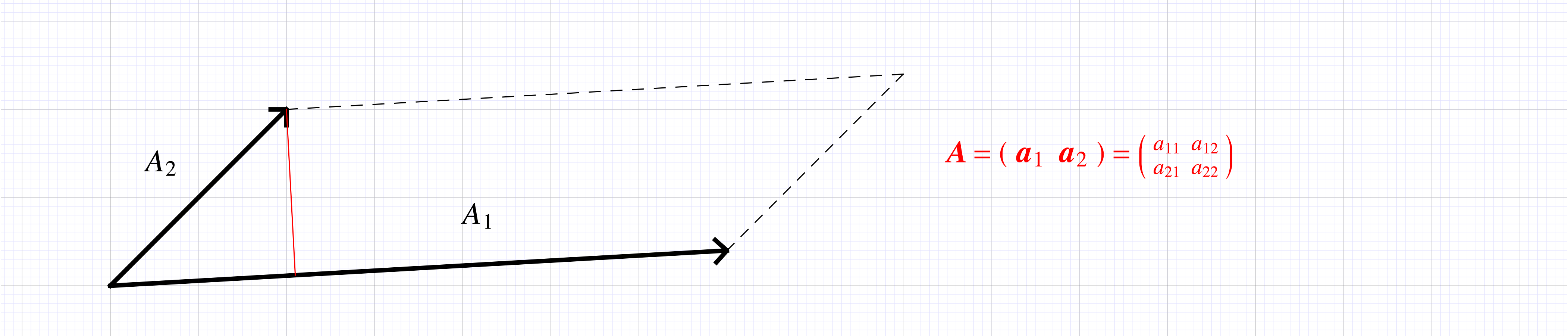
Linear mappings of a vector space onto itself $𝒇:{ℝ}^m\to {ℝ}^m$ are characterized by a square matrix $𝑨\in {ℝ}^{m\times m}$ whose column vectors can be considered as the edges of a geometric object in ${ℝ}^m$. When $m=2$ a parallelogram is obtained with area $S=bh$, with $b$ the length of the base edge and $h$ the height. The parallelogram edges are specified by the vectors ${𝒂}_1,{𝒂}_2$ oriented at angles ${\phi }_1,{\phi }_2$ with respect to the $x_1$$-\mathrm{axis}$. With $\theta ={\phi }_2-{\phi }_1$, the parallelogram height is

${\displaystyle h=||{𝒂}_2||\sin \theta =||{𝒂}_2||\sin .(.{\phi }_2-{\phi }_1)=||{𝒂}_2||(\sin {\phi }_2\cos {\phi }_1-\sin {\phi }_1\cos {\phi }_2).}$

The trigonometric functions can be related to the edge vectors through

${\displaystyle \cos {\phi }_1=a_{11}/||{𝒂}_1||,\sin {\phi }_1=a_{12}/||{𝒂}_1||,\cos {\phi }_2=a_{21}/||{𝒂}_2||,\sin {\phi }_2=a_{22}/||{𝒂}_2||.}$

The above allow statement of a formula for the parallelogram area strictly in terms of edge vector components

${\displaystyle S=||{𝒂}_1||||{𝒂}_2||(\sin {\phi }_2\cos {\phi }_1-\sin {\phi }_1\cos {\phi }_2)=a_{11}{a}_{22}-a_{12}{a}_{21}.}$

By the formula $S$ can be either positive of negative, and indicates the order of denoting edge vectors since the parallelogram can be specified either as edges $\left[\begin{array}{ll}{𝒂}_1& {𝒂}_2\end{array}\right]$ or $\left[\begin{array}{ll}{𝒂}_2& {𝒂}_1\end{array}\right]$.

Figure 1. Area of a parallelogram (hyperparallelipiped in two-dimensions) with edge vectors ${𝒂}_1,{𝒂}_2\in {ℝ}^2$.

Recall that the norm $||𝒗||$ of a vector $𝒗\in {ℝ}^m$ is a functional giving the magnitude of a vector. The norm $||𝑨||$ of a matrix $𝑨\in {ℝ}^{m\times n}$ is also a functional specifying the maximum amplification of vector norm through the linear mapping $𝒇\left(𝒙\right)=𝑨𝒙$, as encountered in the SVD singular values. The above calculations suggest yet another functional, the signed area of the geometric object with edge vectors ${𝒂}_1,\dots ,{𝒂}_m$. This functional is a mapping from the vector space of $m\times m$ matrices $({ℝ}^{m\times m},ℝ,+,\cdot )$ to the reals and is known as the determinant of a matrix.

Definition. The determinant of a square matrix $𝑨=\left[\begin{array}{lll}{𝒂}_1& \dots & {𝒂}_m\end{array}\right]\in {ℝ}^{m\times m}$

${\displaystyle \left|A\right|=\det \left(A\right)=\left|\begin{array}{cccc}{a}_{11}& a_{12}& \dots & a_{1m}\\ a_{21}& a_{22}& \dots & a_{2m}\\ ⋮& ⋮& \ddots & ⋮\\ a_{m1}& a_{m2}& \dots & a_{mm}\end{array}\right|\in ℝ}$

is a real number giving the (oriented) volume of the parallelipiped spanned by matrix column vectors.

The geometric interpretation of a determinant leads to algebraic computation rules. For example, consider the parallelogram with colinear edge vectors, ${𝒂}_2=\alpha {𝒂}_1$. In this case the parallelogram area is zero. In general whenever one of the vectors within $𝒮=\{{𝒂}_1,\dots ,{𝒂}_m\}$ is linearly dependent on the others the dimension of $\mathrm{span}\left(𝒮\right)$ is less than $m$, and the volume of the associated parallelipiped is zero. Deduce that

${\displaystyle 𝑨\in {ℝ}^{m\times m},\mathrm{rank}\left(𝑨\right)<m\Rightarrow \det \left(𝑨\right)=0.}$

(1)

Swapping a pair of edges changes the orientation of the edge vectors and leads to a sign change of the determinant. Another swap changes the sign again. A sign $\sigma \left(P\right)={(-1)}^s$, the parity of a permutation, is associated to any permutation $P$ where $s$ is the number of pair swaps needed to carry out the $P$ permutation. It results that applying a permutation matrix onto $𝑨$ changes the determinant sign

${\displaystyle \det (𝑷𝑨)=\det (𝑨𝑷)=\sigma \left(P\right)\det \left(𝑨\right).}$

(2)

Recall that $𝑷𝑨$ permutes rows and $𝑨𝑷$ permutes columns. The edges of a geometric object could be specified in either column format or row format with no change in the geometric properties leading to

${\displaystyle \det \left(𝑨\right)=\det \left({𝑨}^T\right).}$

(3)

Scaling the length of an edge changes the volume in accordance with

${\displaystyle \det \left[\begin{array}{llll}\alpha {𝒂}_1& {𝒂}_2& \dots & {𝒂}_m\end{array}\right]=\alpha \det \left[\begin{array}{llll}{𝒂}_1& {𝒂}_2& \dots & {𝒂}_m\end{array}\right].}$

(4)

With reference to Fig. (1), consider edge ${𝒂}_1$ decomposed into two parts along the same direction ${𝒂}_1=\alpha {𝒂}_1+(1-\alpha ){𝒂}_1={𝒃}_1+{𝒄}_1$. The area of the parallelogram with edge ${𝒂}_1$ is the sum of those with edges ${𝒃}_1,{𝒄}_1$. This generalizes to arbitrary decompositions of the ${𝒂}_1$ vector, leading to the rule

${\displaystyle \det \left[\begin{array}{llll}{𝒂}_1& {𝒂}_2& \dots & {𝒂}_m\end{array}\right]=\det \left[\begin{array}{llll}{𝒃}_1+{𝒄}_1& {𝒂}_2& \dots & {𝒂}_m\end{array}\right]=\det \left[\begin{array}{llll}{𝒃}_1& {𝒂}_2& \dots & {𝒂}_m\end{array}\right]+\det \left[\begin{array}{llll}{𝒄}_1& {𝒂}_2& \dots & {𝒂}_m\end{array}\right].}$

(5)

The above two rules (4,5) state that the determinant is a linear mapping in the first column. In conjunction with column permutation, deduce that the determinant is linear in any column or row of the matrix $𝑨$. Consider now an important consequence, the result upon the determinant of adding a multiple of one column to another column

${\displaystyle \det \left(\left[\begin{array}{llll}{𝒂}_1+\alpha {𝒂}_2& {𝒂}_2& \dots & {𝒂}_m\end{array}\right]\right)=\det \left(\left[\begin{array}{llll}{𝒂}_1& {𝒂}_2& \dots & {𝒂}_m\end{array}\right]\right)+\alpha \det \left(\left[\begin{array}{llll}{𝒂}_2& {𝒂}_2& \dots & {𝒂}_m\end{array}\right]\right).}$

Since the second term in the above sum has two identical columns its value is zero and

${\displaystyle \det \left(\left[\begin{array}{llll}{𝒂}_1+\alpha {𝒂}_2& {𝒂}_2& \dots & {𝒂}_m\end{array}\right]\right)=\det \left(\left[\begin{array}{llll}{𝒂}_1& {𝒂}_2& \dots & {𝒂}_m\end{array}\right]\right),}$

stating that adding a multiple of a column to another does not change the value of a determinant. Similarly, adding a multiple of a row to another does not change the value of a determinant. The practical importance of the rules is that the elementary operations from Gaussian elimination do not change the value of a determinant.

The determinant of the identity matrix equals one, $\det \left(𝑰\right)=1$, and that of a matrix product is the product of determinants of the factors

${\displaystyle \det (𝑨𝑩)=\det \left(𝑨\right)\det \left(𝑩\right).}$

The determinant of a diagonal matrix $𝑫=\mathrm{diag}(d_1,\dots ,d_m)$ is the product of its diagonal components

${\displaystyle \det \left(𝑫\right)=d_1{d}_2\dots d_m.}$

The properties can be used in conjunction with known matrix factorizations.

1. Determinant of an orthogonal $𝑸$ matrix is $\pm 1$. Since ${𝑸}^T𝑸=𝑰$

   ${\displaystyle \det ({𝑸}^T𝑸)=\det \left({𝑸}^T\right)\det \left(𝑸\right)={\left[\det \left(𝑸\right)\right]}^2=1\Rightarrow \det \left(𝑸\right)=\pm 1.}$

2. Determinant of a matrix equals the product of its singular values

   ${\displaystyle \det \left(𝑨\right)=\det (𝑼𝚺{𝑽}^T)=\det \left(𝑼\right)\det \left(𝚺\right)\det \left({𝑽}^T\right)=\det \left(𝚺\right)={\sigma }_1{\sigma }_2\dots {\sigma }_m.}$

   In particular if $\mathrm{rank}\left(𝑨\right)<m$, $\det \left(𝑨\right)=0$.

The determinant can be defined either in geometric terms as above or in algebraic terms. The ageneral algebraic definition is specified in terms of the components of the matrix $𝑨=\left[a_{ij}\right]$ as

${\displaystyle \det \left(𝑨\right)=\sum _P\sigma \left(P\right)a_{1i_1}{a}_{2i_2}\dots a_{m{i}_m},}$

with the sum carried out over all permutations of $m$ numbers, one of which is specified as

${\displaystyle \left(\begin{array}{llll}1& 2& \dots & m\\ i_1& i_2& \dots & i_m\end{array}\right).}$

There are $m!$ such permuations, a number that grows rapidly with $m$ hence the algebraic definition holds little interest for practical computation, though it was the object of considerable historical interest through Cramer's rule to solve linear systems.

2.Eigenvalues and the characteristic polynomial

The eigenproblem is to find invariant directions of a linear mapping $𝒇:{ℝ}^m\to {ℝ}^m$, meaning those non-zero input vectors that lead to an output in the same direction perhaps scaled by factor $\lambda$

${\displaystyle 𝒇\left(𝒙\right)=\lambda 𝒙,𝑨𝒙=\lambda 𝒙,𝒙\ne 𝟎.}$

The above can be restated as

${\displaystyle (\lambda 𝑰-𝑨)𝒙=𝟎\text{ or }(𝑨-\lambda 𝑰)=𝟎.}$

The above is obviously satisfied for $𝒙=𝟎$, but this case is excluded as a solution to the eigenproblem since the zero vector does not uniquely specify a direction in ${ℝ}^m$. For there to be a non-zero solution to the eigenproblem the null space of $\lambda 𝑰-𝑨$ must be of dimension at least one. It results that the matrix $\lambda 𝑰-𝑨$ is not of full rank, often stated as $\lambda 𝑰-𝑨$ is singular, and at least one of the singular values of $\lambda 𝑰-𝑨$ must be zero. Through the determinant properties it results that

${\displaystyle \det (\lambda 𝑰-𝑨)=0.}$

The algebraic definition of a determinant leads to

${\displaystyle \det (\lambda 𝑰-𝑨)=p\left(\lambda \right)={\lambda }^m+c_{m-1}{\lambda }^{m-1}+\cdots +c_1\lambda +c_0,}$

such that $\det (\lambda 𝑰-𝑨)$ is a polynomial of degree $m$ in $\lambda$. It is known through the fundamental theorem of algebra that a polynomial of degree $m$ has $m$ roots ${\lambda }_1,{\lambda }_2,\dots ,{\lambda }_m\in ℂ$, with some perhaps repeated

${\displaystyle p\left(\lambda \right)=(\lambda -{\lambda }_1)(\lambda -{\lambda }_2)\dots (\lambda -{\lambda }_m).}$

Note that in general the roots can be complex even for polynomials with real coefficients as exemplified by $p\left(\lambda \right)={\lambda }^2+1$. If ${\lambda }_1,{\lambda }_2,\dots ,{\lambda }_K$ are the distinct roots, each repeated $m_1,m_2,\dots ,m_K$ times

${\displaystyle p\left(\lambda \right)={(\lambda -{\lambda }_1)}^{m_1}{(\lambda -{\lambda }_2)}^{m_2}\dots {(\lambda -{\lambda }_K)}^{m_K}.}$

The number of times a root is repeated is called the algebraic multiplicty of an eigenvalue.

For each eigenvalue $𝑨-\lambda 𝑰$ has a non-trivial null space called the eigenspace of $\lambda$

The eigenvector associated with an eigenvalue is a member of this eigenspace

Note that eigenvectors can be scaled by any non-zero number since

In practice, it is customary to enforce $||𝒙||=1$. The dimension of the eigenspace is called the geometric multiplicity of eigenvalue $\lambda$

The conclusion from the above is that $m$ solutions of the eigenproblem exist. There are $m$ eigenvalues, not necessarily distinct, and associated eigenvectors. As usual instead of the individual statements $𝑨{𝒙}_k={\lambda }_k{𝒙}_k$ it is more efficient to group eigenvalues and eigenvectors into matrices

and state the eigenproblem in matrix terms as

3.Eigendecomposition

3.1.Simple cases

Insight into eigenproblem solution is gained by considering common geometric transformations.

Projection matrix. The matrix

projects a vector onto $C\left(𝒒\right)$. Vectors within $C\left(𝒒\right)$ are unaffected $𝑷𝒒=(𝒒{𝒒}^T)𝒒=𝒒\left({𝒒}^T𝒒\right)=𝒒\cdot 1=𝒒$ hence $𝒒$ is an eigenvector with associated eigenvalue $\lambda =1$. The $𝑷$ matrix is of rank one and by the FTLA, $\dim N\left({𝑨}^T\right)=m-1$. In the SVD of $𝑷=𝑼𝚺{𝑽}^T$,

It results that any vector $𝒛$ within the left null space $𝒛\in N\left({𝑷}^T\right)$ is an eigenvector with associated eigenvalue $\lambda =0$. In matrix form the eigenproblem solution is

and since $𝑼$ is orthogonal $𝑼{𝑼}^T=𝑰$, multiplication no the left by ${𝑼}^T$ is possible leading to

Reflection matrix. The matrix

is the reflector across $𝒒$. Vectors colinear with $𝒒$ do not change orientation $𝑹𝒒=𝒒$ and are therefore eigenvectors with associated eigenvalue $\lambda =1$. Vectors $𝒖$ orthogonal to $𝒒$ change orientation along their direction and are hence eigenvectors with associated eigenvalue $\lambda =-1$

In ${ℝ}^m$ there are $m-1$ different vectors orthogonal to $𝒒$ and mutually orthonormal. The eigenproblem solution can again be stated in matrix form as

Since $𝑼$ is an orthogonal matrix, it results that

Rotation matrix. The matrix

represents the isometric rotation of two-dimensional vectors. If $\theta =0$, $𝑹=𝑰$ with eigenvalues ${\lambda }_1={\lambda }_2=1$, and eigenvector matrix $𝑿=𝑰$. For $\theta =\pi$, the eigenvalues are ${\lambda }_1={\lambda }_2=-1$, again with eigenvector matrix $𝑿=𝑰$. If $\sin \theta \ne 0$, the orientation of any non-zero $𝒙\in {ℝ}^2$ changes upon rotation by $\theta$. The characteristic polynomial has complex roots

and the directions of invariant orientation have complex components (are outside the real plane ${ℝ}^2$)

3.2.Vectors and matrices with complex components

The above rotation case is an example of complex values arising in the solution of an eigenproblem for a matrix with real coefficients. Fortunately, the framework for working with vectors and matrices that have complex components is almost identical to working in the reals. The only significant difference is the realtionship between the two-norm and inner product. When $𝒖,𝒗\in {ℝ}^m$ the inner product ${𝒖}^T𝒗$ corresponds to the dot product and the two-norm of a vector can be defined as

Consider a complex number $z=x+iy$, taken to represent a point at coordinates $(x,y)$in the ${ℝ}^2$ plane. The magnitude or absolute value of $z$ is defined as the distance from the origin to point $(x,y)$ in ${ℝ}^2$

Introducing the complex conjugate $\bar{z}=x-iy$ (the reflection of $(x,y)$ across the $x$-axis), the absolute value can also be stated as

Extending this idea to vectors of complex numbers, transposition is combined with taking the conjugate into an operation of taking the adjoint denoted by an $\ast$ superscript

Everywhere a transposition appears when dealing with vectors in ${ℝ}^m$, it is replaced by taking the adjoint when working with vectors in ${ℂ}^m$. Most notably when $𝑼\in {ℝ}^{m\times m}$ it is said to be orthogonal if

For $𝑼\in {ℂ}^{m\times m}$ the matrix is said to be unitary if

Orthogonality of $𝒖,𝒗\in {ℂ}^m$ is expressed as ${𝒖}^{\ast }𝒗=0$. The FTLA is restated as

and the SVD as

3.3.General solution of the eigenproblem

As exemplified above, solving an eigenproblem $𝑨𝒙=\lambda 𝒙,𝑨\in {ℝ}^{m\times m}$ requires:

1. Finding the roots ${\lambda }_1,\dots ,{\lambda }_m$of the characteristic polynomial $p\left(\lambda \right)=\det (\lambda 𝑰-𝑨)$;

2. Finding bases for the eigenspaces $E_{{}_k}=N(𝑨-{\lambda }_k𝑰)$.

The matrix form of the solution is then stated as

If the matrix $𝑿$ has linearly independent columns (it is non-singular), it can then be inverted leading to the eigendecomposition

yet another factorization of the matrix $𝑨$. Such eigendecompositions are very useful when repeatedly applying a linear mapping since $𝒇\left(𝒇\left(𝒙\right)\right)=𝒇(𝑨𝒙)={𝑨}^2𝒙$. In general after $k$ applications of $𝒇$ the matrix ${𝑨}^k$ arises. If an eigendecomposition is avaiable, then

and ${𝚲}^k$ is easily computable

The simple eigenproblem for

reveals issues that might arise in more general situations. The characteristic polynomial

has a repeated root ${\lambda }_1={\lambda }_2=1$. Note that

is already in row echelon form indicating that $\mathrm{rank}(𝑨-{\lambda }_1𝑰)=1$. The FTLA then states the

and the matrix form of the eigenproblem solution is

Note that the second column of $𝑿$ is the same as the first, hence $𝑿$ has linearly dependent columns and cannot be inverted. The matrix $𝑨$ has an eigenproblem solution but does not have an eigendecomposition. An eigendecomposition is possible only when for each eigenvalue its algebraic multiplicty is equal to its geometric multiplicity.

An immediate question is to identify those matrices for which an eigendecomposition is possible and perhaps of a particularly simple form. A matrix $𝑨\in {ℂ}^{m\times m}$ is said to be normal if

A normal matrix has a unitary eigendecomposition. There exists $𝑸\in {ℂ}^{m\times m}$ unitary that satisfies

In the real case the above becomes $𝑨{𝑨}^T={𝑨}^T𝑨$, and there exists $𝑸\in {ℝ}^{m\times m}$ orthogonal that satisfies

Computational procedures to solve an eigenproblem become quite complicated for the general case and have been the object of extensive research. Fortunately the problem is well understood and solution procedures have been implemented in all major computational systems. In Julia for example:

∴ 

A=[1 0; 0 2]; eigvals(A)

∴ 

eigvecs(A)

∴ 

A=[1 1; 0 1]; eigvals(A)

∴ 

eigvecs(A)

∴ 

4.Finding the SVD

An important application of eigendecompositions is actual computation of the SVD. The SVD theorem simply asserted existence of intrinsic orthogonal basis for the domain and codomain of a linear mapping in which the mapping behaved as a simple scaling. It did not provide a procedure to find those bases in general.

From the above, though an eigendecomposition for general $𝑨\in {ℝ}^{m\times n}$ may not exist, an orthogonal decomposition always exists for $𝑩=𝑨{𝑨}^T$ since

verifies that $𝑩$ is normal. Consider now the SVD $𝑨=𝑼𝚺{𝑽}^T$ to find that

stating that the left singular vectors $𝑼$ are the eigenvectors of $𝑨{𝑨}^T$. Likewise $𝑪=𝑨{}^T𝑨$ is a normal matrix and from

the right singular vectors are found as the eigenvectors of $𝑨{}^T𝑨$. The singular values of $𝑨$ are the square roots of the eigenvalues of either $𝑩$ or $𝑪$.

The two eigenproblems above are solved whenever a computation of the SVD is invoked within Julia.