MATH347DS L06: The singular value decomposition

Overview

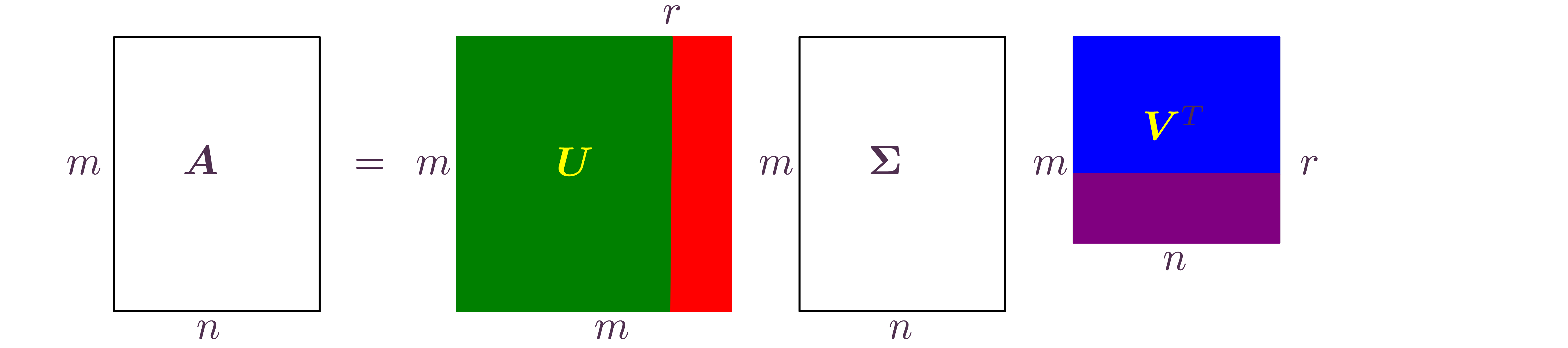
• The singular value decomposition (SVD)

  • Motivation

  • Theorem

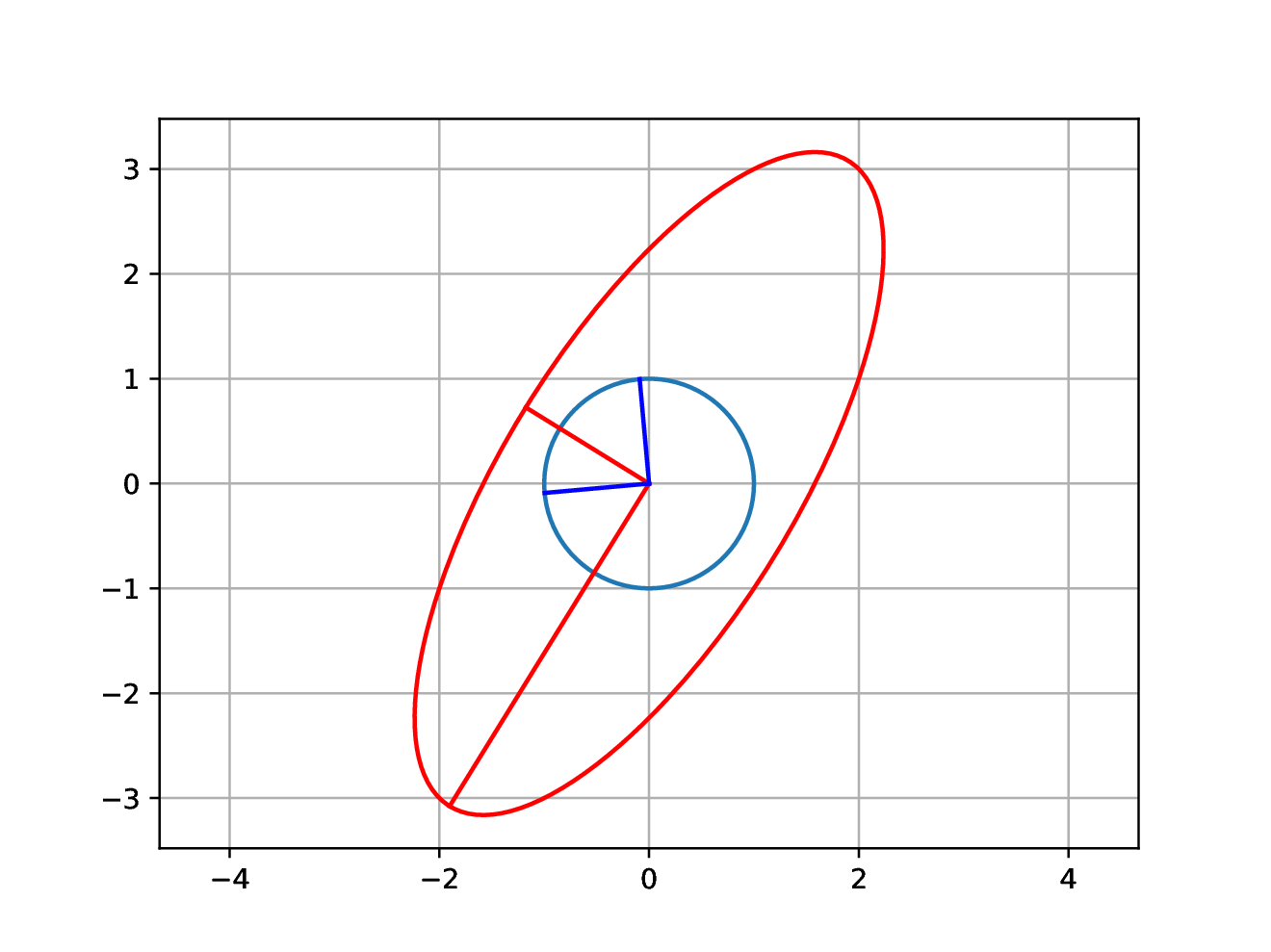
• Another essential diagram: SVD finds orthonormal bases for $C\left(𝑨\right),N\left({𝑨}^T\right),C\left({𝑨}^T\right),N\left(𝑨\right)$

• SVD computation

• Rank-1 expansion of a matrix

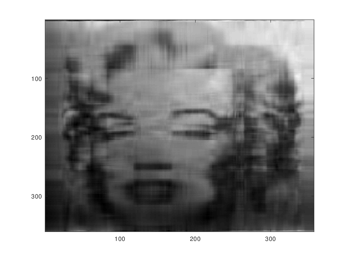
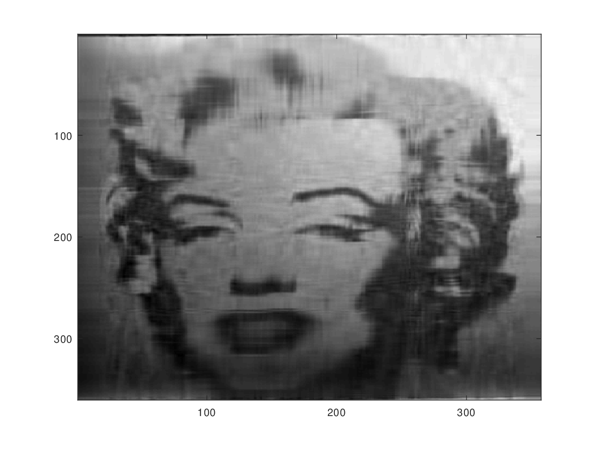
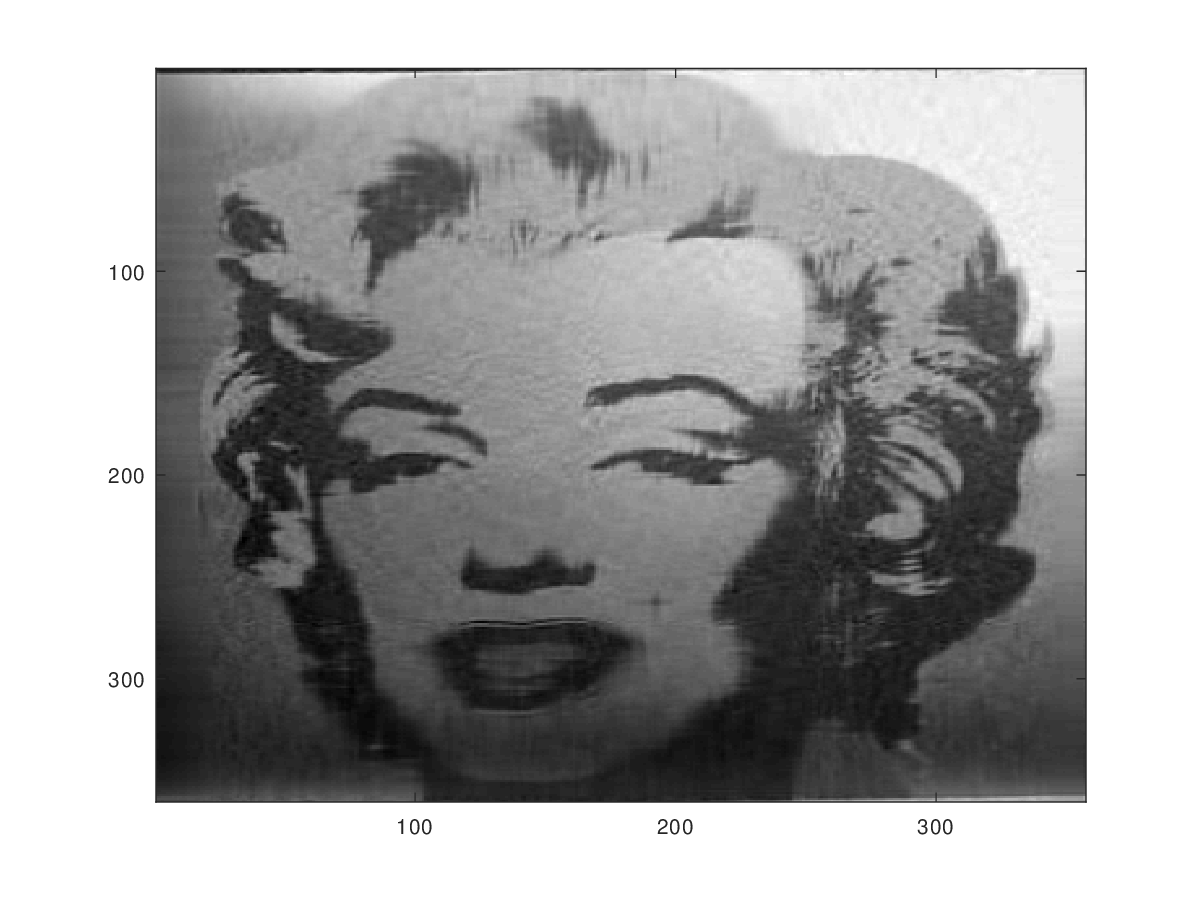
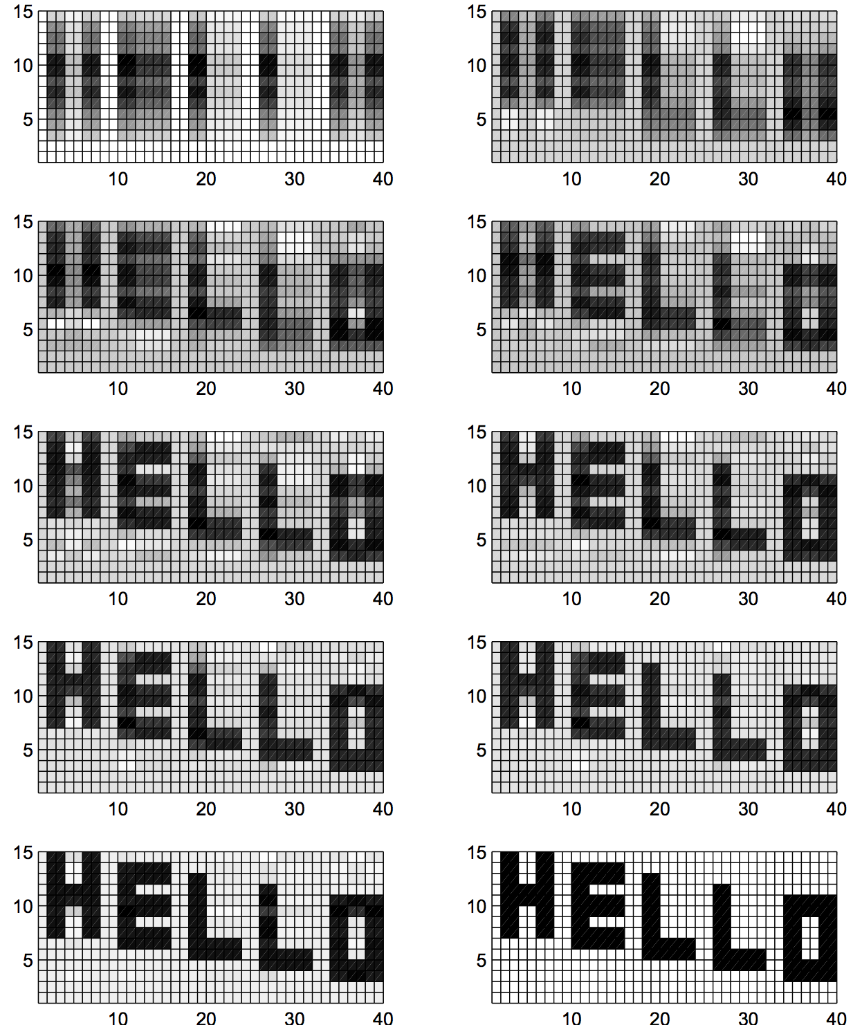
• SVD in image compression, analysis

• The pseudo-inverse

Motivation singular value decomposition (SVD)

• Motivation: FTLA does not specify bases for $C\left(𝑨\right),N\left({𝑨}^T\right),C\left({𝑨}^T\right),N\left(𝑨\right)$.

• Question: Is there some “natural” basis for the fundamental matrix subspaces?

• Consider linear mapping: $𝒇:{ℝ}^n\to {ℝ}^m$, $𝒇\left(𝒙\right)=𝑨𝒙$, $𝑨\in {ℝ}^{m\times n}$

  • The input $𝒙$ is given in the identity matrix basis, $𝒙={𝑰}_n𝒙$

  • The output $𝒃=𝒇\left(𝒙\right)=𝑨𝒙$ is also obtained in the identity matrix basis, $𝒚={𝑰}_m𝒚$

  • In these basis the effect of $𝑨$ might be costly to compute

    ${\displaystyle 𝒃=x_1{𝒂}_1+x_2{𝒂}_2+\cdots +x_n{𝒂}_n\Rightarrow b_i=x_1{a}_{i1}+x_2{a}_{i2}+\cdots +x_n{a}_{i,n}.}$

  • What would be simpler? One possibility: a simple scaling of each component suggested by

    ${\displaystyle 𝒃=\left[\begin{array}{l}{b}_1\\ b_2\\ ⋮\\ b_m\end{array}\right]=𝑫𝒙=\mathrm{diag}({\lambda }_1,{\lambda }_2,\dots ,{\lambda }_m)𝒙=\left[\begin{array}{llll}{\lambda }_1& 0& \dots & 0\\ 0& {\lambda }_2& \dots & 0\\ ⋮& ⋮& \ddots & ⋮\\ 0& 0& \dots & {\lambda }_m\end{array}\right]\left[\begin{array}{l}{x}_1\\ x_2\\ ⋮\\ x_m\end{array}\right]\Rightarrow b_i={\lambda }_i{x}_i}$

Stating desired behavior

• Seek different bases for domain, codomain of $𝒇:{ℝ}^n\to {ℝ}^m$, $𝒇\left(𝒙\right)=𝑨𝒙$, $𝑨\in {ℝ}^{m\times n}$

  • an orthonormal basis $𝑽$ in ${ℝ}^n$, $𝑽\in {ℝ}^{n\times n}$, $𝑽{𝑽}^T={𝑽}^T𝑽={𝑰}_n$

    ${\displaystyle 𝑰𝒙=𝑽𝒚\Rightarrow 𝒚={𝑽}^T𝒙}$

  • an orthonormal basis $𝑼$ in ${ℝ}^m$, $𝑼\in {ℝ}^{m\times m}$, $𝑼{𝑼}^T={𝑼}^T𝑼={𝑰}_m$

    ${\displaystyle 𝑰𝒃=𝑼𝒄\Rightarrow 𝒄={𝑼}^T𝒃}$

  • impose that the effect of $𝑨$ in the new bases is a simple component scaling

    ${\displaystyle 𝒄=𝚺𝒚\Rightarrow {𝑼}^T𝒃=𝚺{𝑽}^T𝒙\Rightarrow 𝒃=𝑼𝚺{𝑽}^T𝒙\Rightarrow }$ ${\displaystyle 𝑨=𝑼𝚺{𝑽}^T}$

  • Note that $𝚺\in {ℝ}^{m\times n}$

Can it be done? Yes: Singular value decomposition theorem

Theorem. (SVD) For any $𝑨\in {ℝ}^{m\times n}$, $𝑨=𝑼𝚺{𝑽}^T$, with $𝑼\in {ℝ}^{m\times m}$, $𝑽\in {ℝ}^{n\times n}$ orthogonal, $𝚺\in {ℝ}_{+}^{m\times n}$ pseudo-diagonal $𝚺=\mathrm{diag}({\sigma }_1,\dots ,{\sigma }_r,\dots ,0)$, ${\sigma }_1⩾{\sigma }_2⩾\cdots ⩾{\sigma }_r>0$, $r⩽min(m,n)$

The SVD is determined by eigendecomposition of ${𝑨}^T𝑨$, and $𝑨{𝑨}^T$

• ${𝑨}^T𝑨={(𝑼𝚺{𝑽}^T)}^T(𝑼𝚺{𝑽}^T)=𝑽({𝚺}^T𝚺){𝑽}^T$, an eigendecomposition of ${𝑨}^T𝑨$. The columns of $𝑽$ are eigenvectors of ${𝑨}^T𝑨$ and called right singular vectors of $𝑨$

• $𝑨{𝑨}^T=(𝑼𝚺{𝑽}^T){(𝑼{𝚺}^T{𝑽}^T)}^T=𝑼\left(𝚺{𝚺}^T\right){𝑼}^T$, an eigendecomposition of $𝑨{𝑨}^T$. The columns of $𝑼$ are eigenvectors of $𝑨{𝑨}^T$ and called left singular vectors of $𝑨$

• The matrix $𝚺$ has zero elements except for the diagonal that contains ${\sigma }_i$, the singular values of $𝑨$, computed as the square roots of the eigenvalues of ${𝑨}^T𝑨$ (or $𝑨{𝑨}^T$)

An all-encompassing diagram: SVD and matrix subspaces

• SVD of $𝑨\in {ℝ}^{m\times n}$ reveals: $\mathrm{rank}\left(𝑨\right)$, bases for $C\left(𝑨\right),N\left({𝑨}^T\right),C\left({𝑨}^T\right),N\left(𝑨\right)$

SVD Computation

• From $𝑨=𝑼𝚺{𝑽}^T$ deduce $𝑨{𝑨}^T=𝑼{𝚺}^2{𝑼}^T$, $𝑨{}^T𝑨=𝑽{𝚺}^2{𝑽}^T$, hence $𝑼$ is the eigenvector matrix of $𝑨{𝑨}^T$, and $𝑽$ is the eigenvector matrix of ${𝑨}^T𝑨$

• SVD computation is available in Julia, Octave, Matlab, Mathematica ...

  ∴	short(x) = round(x,digits=6);

  ∴	A=[2 -1; -3 1]; F=svd(A); U=F.U; Σ=Diagonal(F.S); Vt=F.Vt; short.([A U*Σ*Vt])

  ${\displaystyle \left[\begin{array}{cccc}2.0& -1.0& 2.0& -1.0\\ -3.0& 1.0& -3.0& 1.0\end{array}\right]}$

  (1)

  ∴	short.([U Σ Vt'])

  ${\displaystyle \left[\begin{array}{cccccc}-0.576048& 0.817416& 3.864328& 0.0& -0.932722& -0.360597\\ 0.817416& 0.576048& 0.0& 0.258777& 0.360597& -0.932722\end{array}\right]}$

  (2)

  ∴

• SVD of $𝑨=\left[\begin{array}{ll}2& -1\\ 3& 1\end{array}\right]$ diagram, $𝒇\left(𝒙\right)=𝑨𝒙$

  

Additive decomposition of $𝑨$

• $𝑨=𝑼𝚺{𝑽}^T$, carry out block multiplication

  ${\displaystyle 𝑨=\left[\begin{array}{llllll}{𝒖}_1& \dots & {𝒖}_r& {𝒖}_{r+1}& \dots & {𝒖}_m\end{array}\right]\left[\begin{array}{lllll}{\sigma }_1& & & & \\ & \ddots & & & \\ & & {\sigma }_r& & \\ & & & 0& \\ & & & & \ddots \end{array}\right]\left[\begin{array}{l}{{𝒗}_1}^T\\ ⋮\\ {{𝒗}_r}^T\\ {{𝒗}_{r+1}}^T\\ ⋮\\ {{𝒗}_n}^T\end{array}\right]\Rightarrow }$ ${\displaystyle 𝑨=\left[\begin{array}{llllll}{𝒖}_1& \dots & {𝒖}_r& {𝒖}_{r+1}& \dots & {𝒖}_m\end{array}\right]\left[\begin{array}{l}{\sigma }_1{{𝒗}_1}^T\\ ⋮\\ {\sigma }_r{{𝒗}_r}^T\\ 𝟎\\ ⋮\\ 𝟎\end{array}\right]={\sigma }_1{𝒖}_1{𝒗}_1^T+\dots +{\sigma }_r{𝒖}_r{𝒗}_r^T}$

• The above is known as a “rank-one” expansion since $\mathrm{rank}\left({𝒖}_k{𝒗}_k^T\right)=1$. Note that ${𝒖}_k{𝒗}_k^T\in {ℝ}^{m\times n}$ and is a matrix whose columns are $n$ scalings of ${𝒖}_k$

• SVD theorem: ${\sigma }_1⩾{\sigma }_2⩾\cdots ⩾{\sigma }_r>0$, Often ${\sigma }_1⩾{\sigma }_2⩾\cdots ⩾{\sigma }_k\gg {\sigma }_{k+1}⩾\cdots ⩾{\sigma }_r>0$

Low-rank matrix approximation

• Full SVD

  ${\displaystyle 𝑨=\sum _{i=1}^r{\sigma }_i{𝒖}_i{𝒗}_i^T,r⩽min(m,n).}$

• Truncated SVD

  ${\displaystyle 𝑨\cong {𝑨}_p=\sum _{i=1}^p{\sigma }_i{𝒖}_i{𝒗}_i^T.}$

• Many applications, e.g., image compression

Why does SVD image compression work?

• Consider $x_1,x_2:ℝ\to ℝ$, data streams in time of inputs $x_1\left(t\right)$ and outputs $x_2\left(t\right)$

• Is there some function $f$ linking outputs to inputs? $f\left(x_1\left(t\right)\right)=x_2\left(t\right)$

• Seek answer by first asking: is $x_2$ correlated to $x_1$?

• Introduce mean values

  ${\displaystyle {\mu }_1\cong {\bar{x}}_1=\frac{1}{N}\sum _{i=1}^N{x}_1\left(t_i\right)=E\left[x_1\right],{\mu }_2\cong {\bar{x}}_2=\frac{1}{N}\sum _{i=1}^N{x}_2\left(t_i\right)=E\left[x_2\right].}$

• $E$ is the expectation, a linear mapping, $E:{ℝ}^N\to ℝ$ whose associated matrix is

  ${\displaystyle 𝑬=\frac{1}{N}\left[\begin{array}{cccc}1& 1& \dots & 1\end{array}\right].}$

• Shift data such that ${\bar{x}}_1={\bar{x}}_2=0$. Define correlation coefficient

  ${\displaystyle \rho (x_1,x_2)=\frac{E\left[x_1{x}_2\right]}{{\sigma }_1{\sigma }_2}=\frac{E\left[x_1{x}_2\right]}{\sqrt{E\left[x_1^2\right]E\left[x_2^2\right]}}=\frac{{𝒙}_1^T{𝒙}_2}{{||{𝒙}_1||}_{}{||{𝒙}_2||}_{}}.}$

• uncorrelated, if $\rho =0$; correlated, if $\rho =1$; anti-correlated, if $\rho =-1$.

Examples

• Correlated signals

  ∴	t=0:0.01:1; x1=1.0*t; x2=t.^2; rho=transpose(x1)*x2/norm(x1)/norm(x2)

  $0.968249831385581$

  ∴

• Uncorrelated signals

  ∴	m=size(x1)[1]; x3=2*(rand(m,1).-0.5)[:,1]; rho=transpose(x1)*x3/norm(x1)/norm(x3)

  $0.040354121344516436$

  ∴

• Anticorrelated signals

  ∴	x4=-t.^2; rho=transpose(x1)*x4/norm(x1)/norm(x4)

Extend correlation to input, output vectors

• Are input and output parameters $𝒙\in {ℝ}^n$, $𝒚\in {ℝ}^m$ well chosen?

• Perhaps components are redundant, a more economical description might be

  ${\displaystyle 𝒖\in {ℝ}^q,𝒗\in {ℝ}^p,p<m,q<n}$

• Extend idea from correlation coefficient: take $N$ measurements

  ${\displaystyle 𝑿=\left[\begin{array}{cccc}{𝒙}_1& {𝒙}_2& \dots & {𝒙}_n\end{array}\right]\in {ℝ}^{N\times n},𝒀=\left[\begin{array}{cccc}{𝒚}_1& {𝒚}_2& \dots & {𝒚}_n\end{array}\right]\in {ℝ}^{N\times m}.}$

• Choose origin such that $E\left[𝒙\right]=𝟎,E\left[𝒚\right]=𝟎.$

• Covariance matrix (generalization of single variable variance)

  ${\displaystyle {𝑪}_{𝑿}={𝑿}^T𝑿=\left[\begin{array}{c}{𝒙}_1^T\\ {𝒙}_2^T\\ ⋮\\ {𝒙}_n^T\end{array}\right]\left[\begin{array}{cccc}{𝒙}_1& {𝒙}_2& \dots & {𝒙}_n\end{array}\right]=\left[\begin{array}{cccc}{𝒙}_1^T{𝒙}_1& {𝒙}_1^T{𝒙}_2& \dots & {𝒙}_1^T{𝒙}_n\\ {𝒙}_2^T{𝒙}_1& {𝒙}_2^T{𝒙}_2& \dots & {𝒙}_2^T{𝒙}_n\\ ⋮& ⋮& \ddots & ⋮\\ {𝒙}_n^T{𝒙}_1& {𝒙}_n^T{𝒙}_2& \dots & {𝒙}_n^T{𝒙}_n\end{array}\right]}$

Reduced description by truncation of covariance matrix SVD

• SVDs: $𝑿=𝑼𝚺{𝑽}^T$, $C_{𝑿}={𝑿}^T𝑿=𝑽𝚲{𝑽}^T$, $𝚲={𝚺}^T𝚺$

• Take first $q$ column vectors of $𝑽$, ${𝑽}_q=\left[\begin{array}{lll}{𝒗}_1& \dots & {𝒗}_q\end{array}\right]$, $q<n$

  ${\displaystyle 𝒙={𝑽}_q𝒖=\left[\begin{array}{cccc}{𝒗}_1& {𝒗}_2& \dots & {𝒗}_q\end{array}\right]𝒖.}$

• System description in terms of $𝒖\in {ℝ}^q$ is more economical than that in terms of $𝒙\in {ℝ}^n$

• In image compression, successive pixel columns are correlated and reduced descriptions are possible

SVD solution of linear algebra problems: linear systems, least squares

• Consider linear system $𝑨𝒙=𝒃$, $𝑨\in {ℝ}^{m\times m}$, $\mathrm{rank}\left(𝑨\right)=m$. SVD solution steps:

1. Compute the SVD, $𝑼𝚺{𝑽}^T=𝑨$;

2. Find the coordinates of $𝒃$ in the orthogonal basis $𝑼$, $𝒄={𝑼}^T𝒃$;

3. Scale the coordinates of $𝒄$ by the inverse of the singular values $y_i=c_i/{\sigma }_i$, $i=1,\dots ,m$, such that $\Sigma 𝒚=𝒄$ is satisfied;

4. Find the coordinates of $𝒚$ in basis ${𝑽}^T$, $𝒙=𝑽𝒚$.

• What if $𝑨\in {ℝ}^{m\times n}$, $\mathrm{rank}\left(𝑨\right)=r<m$. If $𝒃\in C\left(𝑨\right)$ above procedure still works with a simple modification of step 3 with $i$ going now from 1 to $r$

1. $𝑼𝚺{𝑽}^T=𝑨$;

2. $𝒄={𝑼}^T𝒃$;

3. $y_i=c_i/{\sigma }_i$, $i=1,\dots ,r$

4. $𝒙=𝑽𝒚$.

• If $𝑨\in {ℝ}^{m\times n}$, $\mathrm{rank}\left(𝑨\right)=r<m$. If $𝒃\notin C\left(𝑨\right)$, the above steps give the best approximation of $𝒃$ by linear combination of columns of $𝑨$ in the 2-norm

Pseudo-inverse matrix

• Since the steps to solve a linear system or find best approximation are identical define a matrix ${𝑨}^{+}$ that carries out all steps:

  ${\displaystyle (𝑼𝚺{𝑽}^T)𝒙=𝒃\iff 𝑼(𝚺{𝑽}^T𝒙)=𝒃}$ ${\displaystyle (𝚺{𝑽}^T𝒙)={𝑼}^T𝒃\iff 𝚺({𝑽}^T𝒙)={𝑼}^T𝒃}$

• Recall $𝚺=\mathrm{diag}({\sigma }_1,{\sigma }_2,\dots ,{\sigma }_r,0,\dots 0)$. Define ${𝚺}^{+}=$$\mathrm{diag}(1/{\sigma }_1,1/{\sigma }_2,\dots ,1/{\sigma }_r,0,\dots 0)$

  ${\displaystyle {𝑽}^T𝒙={𝚺}^{+}{𝑼}^T𝒃}$ ${\displaystyle 𝒙=𝑽{𝚺}^{+}{𝑼}^T𝒃}$

• Gather all above steps into a single matrix ${𝑨}^{+}=𝑽{𝚺}^{+}{𝑼}^T$ called the pseudo-inverse of $𝑨$.

• The solution then to a linear system (either exact solution of best approximation) is

  ${\displaystyle 𝒙={𝑨}^{+}𝒃}$

• In Julia, Matlab, Octave, above procedure is implemented through x=A\b.