MATH383: A first course in differential equationsMay 1, 2020

Solve the following problems (4 course points each). Present a brief motivation of your method of solution. Explicitly state any conditions that must be met for solution procedure to be valid. Organize your computation and writing so the solution you present is readily legible. No credit is awarded for statement of the final answer to a problem without presentation of solution procedure.

This is an open-book test, and you are free to consult the textbook or use software to check your solution. Your submission must however reflect your individual effort with no aid from any other person. If you studied the course material and understood solutions to the homework assignments, drafting examination question solutions in TeXmacs should take about 60 minutes. The questions test insight into course theoretical material and do not require extensive calculations. The allotted time is 3 hours, thus also providing flexibility for internet connection interruption and special needs accomodation.

Draft your solution in TeXmacs in this file. Upload your answer into Sakai. Allow at least 10 minutes before the submission cut-off time to ensure you can upload your file.

Problem 1

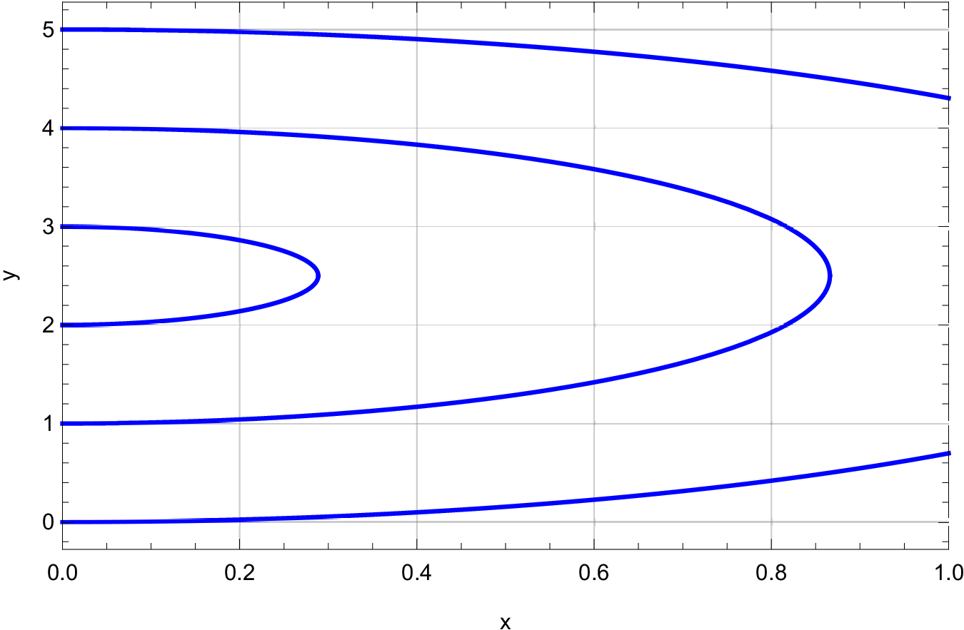
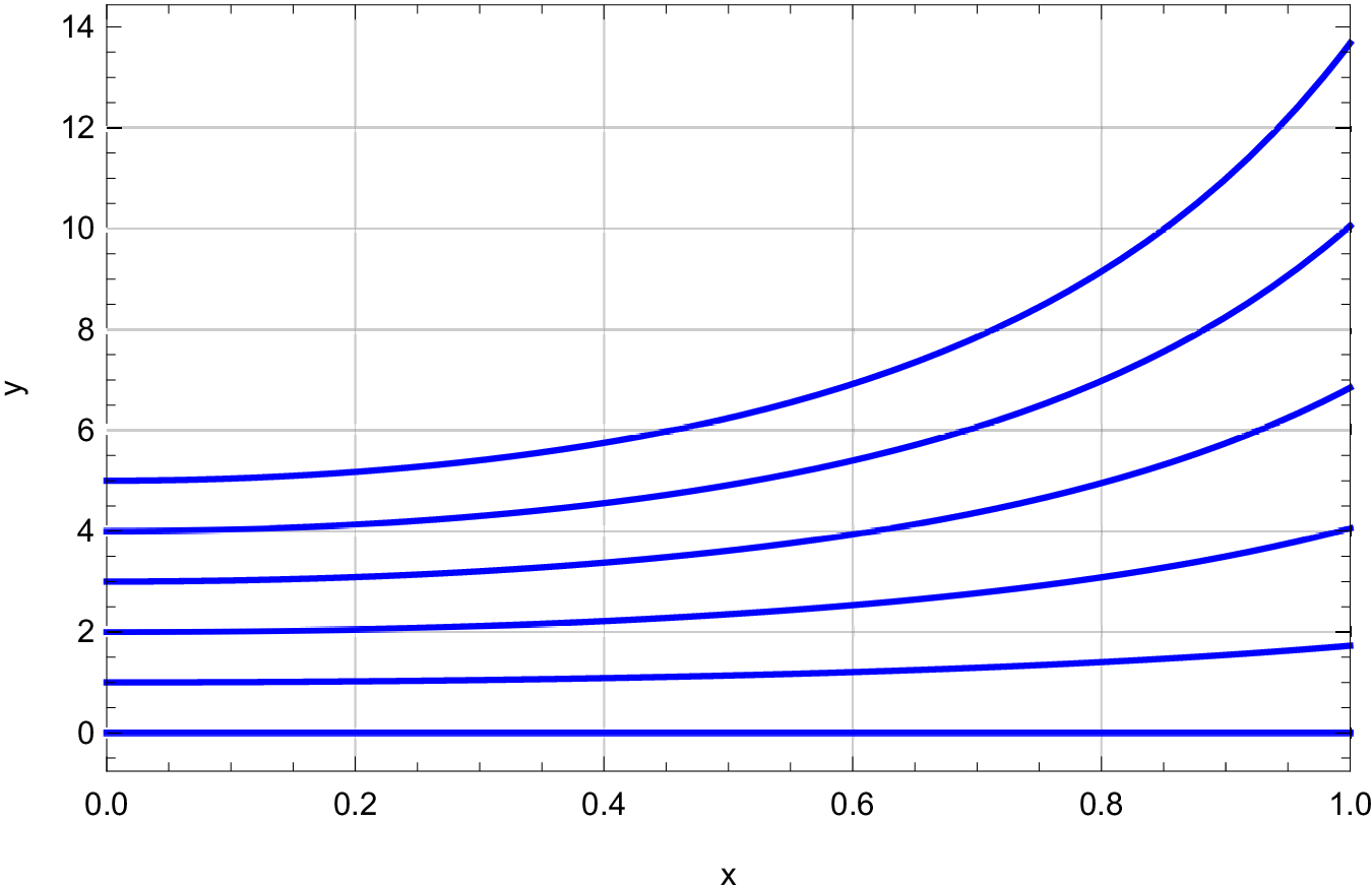
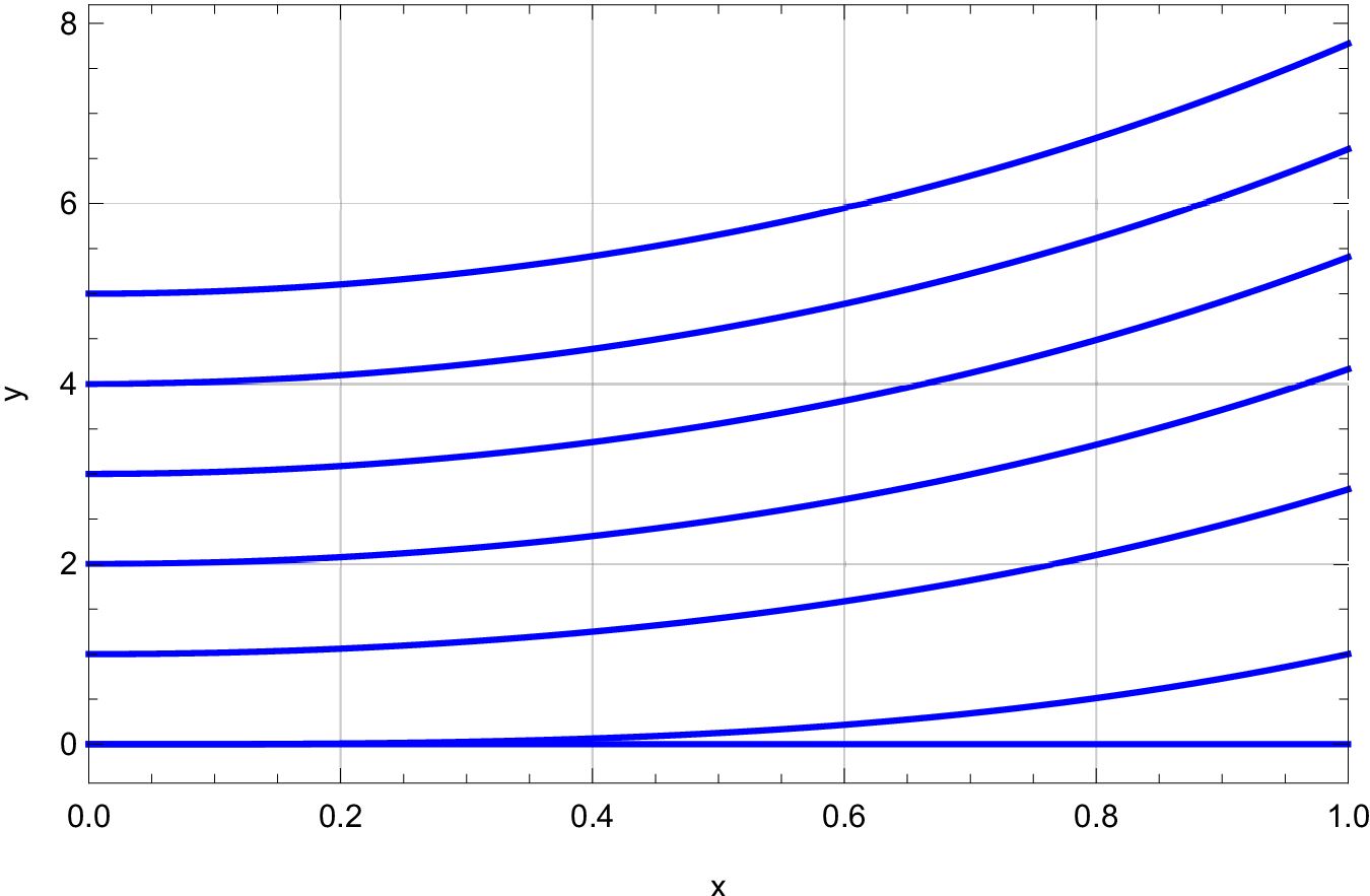
Consider the following differential equations:

1. $y^{\text{'}}=a(x,y)=3x{y}^{4/3}$ ;

2. $y^{\text{'}}=b(x,y)=3x{y}^{1/3}$ ;

3. $y^{\text{'}}=c(x,y)=6x/(5-2y)$.

Figures 1-3 show solutions to the initial value problems $y\left(0\right)$ $\in \{0,1,2,3,4,5\}$, for each of the above equations. Match each equation to a figure. Present the theoretical basis for the matching you present.

Figure 1.

Figure 2.

Figure 3.

Solution. There are $n=6$ initial conditions. Figure 3 shows seven plots, hence admits multiple solutions for initial condition $(x_0,y_0)=(0,0)$, possible when $f_y=\partial f/\partial y$ is not continuous for a differential equation $y^{\text{'}}=f(x,y)$. This corresponds to $b_y(x,y)=x/y^{2/3}$, so $y^{\text{'}}=b(x,y)$ matches with Figure 3. Figure 1 shows trajectories that meet at $y=2.5$, possible only for $y^{\text{'}}=c(x,y)$ with $c_y=12x/(5-2y)$, discontinuous at $y=5/2$. Figure 2 shows 6 non-intersecting trajectories, and corresponds to $y^{\text{'}}=a(x,y)$ with $a(x,y)$ continuous, and $a_y$ continuous for $y⩾0$.

Problem 2

1. Write the exact differential that corresponds to the implicit solution $F(x,y)=xy=1$.

2. Determine $f(x,y)$ that re-expresses the exact differential as an explicit differential equation $y^{\text{'}}=f(x,y)$.

3. Classify the differential equation $y^{\text{'}}=f(x,y)$ according to all criteria you know.

4. Solve the initial value problem $y^{\text{'}}=f(x,y)$, $y\left(1\right)=c$.

Solution.

1. Take differential $dF=F_{x}dx+F_{y}dy=ydx+xdy$=0.

2. From above, obtain

   ${\displaystyle y^{\text{'}}=\frac{dy}{dx}=-\frac{y}{x}=f(x,y).}$

   (1)

3. Equation 1 is a linear, homogeneous, separable, first-order differential equation with $f$ continuous in $y$ and $f_y$ continuous, and admits a unique solution for any initial condition $(x_0,y_0)$, except for $(0,0)$.

4. By direct integration

   ${\displaystyle \frac{dy}{y}=-\frac{dx}{x}\Rightarrow \ln y=-\ln x+\ln C\Rightarrow xy=C,}$

   and for $y\left(1\right)=c$, obtain $xy=c$.

Problem 3

At $t=0$, a system at its equilibrium position is imparted a velocity $v=1$. The plot of the system trajectory $y\left(t\right)$ is rendered in Figure 4, and exhibits inertia, dissipation and storage. Write a differential equation describing the system with numerical coefficients deduced from the plotted trajectory.

Figure 4.

Solution. A system with inertia, dissipation and storage obeys a second-order differential equation $A(t,y,y^{\text{'}})y^{\text{'}\text{'}}+B(t,y,y^{\text{'}})y^{\text{'}}+C(t,y,y^{\text{'}})y=0$. Make hypothesis that equation is linear with constant coefficients

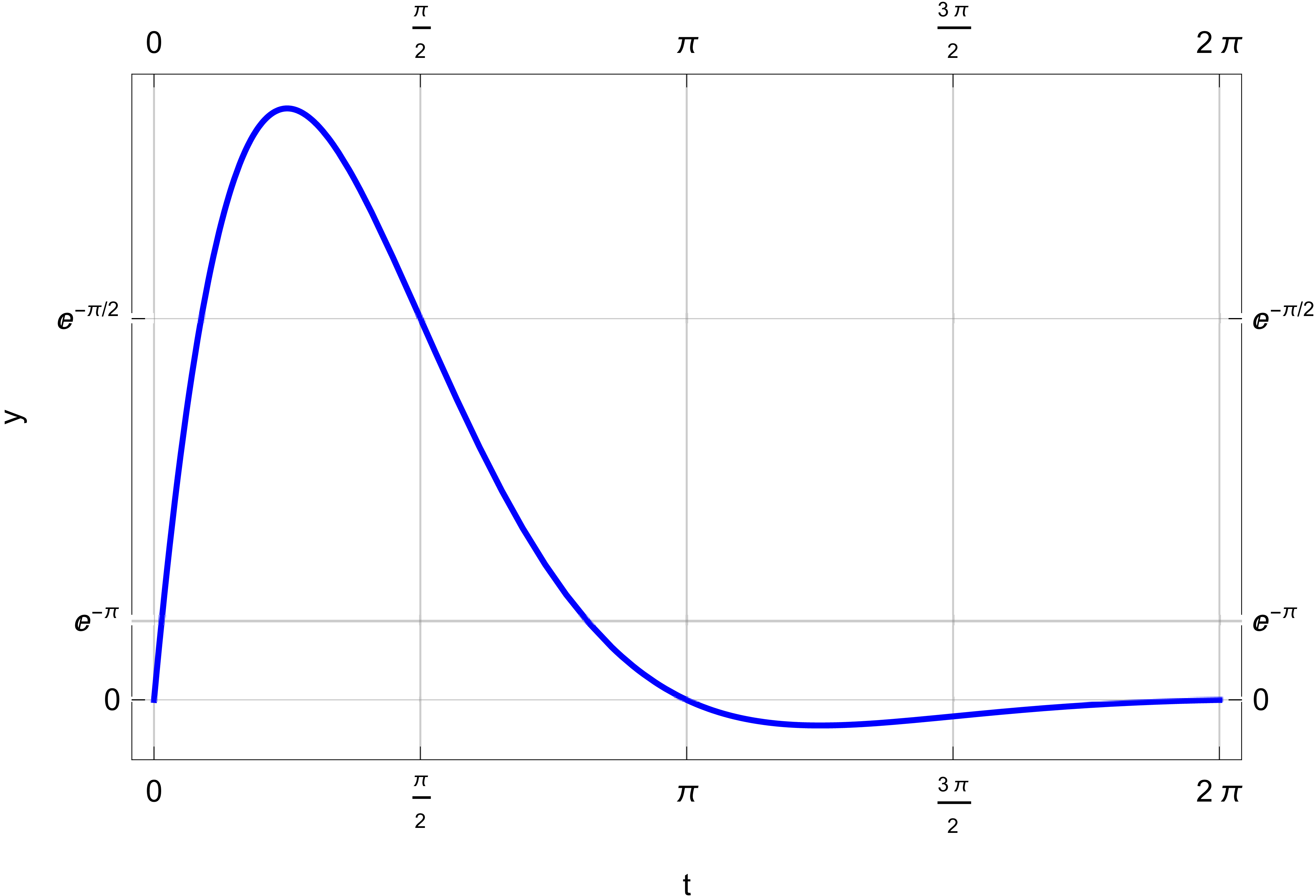with $m,c,k>0$ (problems states inertia, dissipation and storage are present). Choose units such that $m=1$, to rewrite equation as $y^{\text{'}\text{'}}+2c{y}^{\text{'}}+ky=0$, and upon trying solutions of form $y=e^{rt}$, obtain quadratic characteristic equation

with solutions

Figure 4 indicates an underdamped system that suggests $c^2<k$, and introducing $\omega =i\sqrt{k-c^2}$, the general solution would be

From Figure 4, $y\left(0\right)=0$ implies $y\left(0\right)=A=0$. From Figure 4 $y\left(\pi \right)=0$, implies $y\left(\pi \right)=e^{-c\pi }\sin (\omega \pi )=0$, so $\omega$ must be an integer. Since $e^{-ct}$ is continuous, monotonic decreasing, and Figure 4 shows a single maximum between $t=0$ and $t=\pi$, it results that $\omega =1$ (any other integer would produce multiple extrema between $t=0$ and $t=\pi$), hence

Finally, $y(\pi /2)=e^{-c\pi /2}\sin (\pi /2)=e^{-\pi /2}$ from Figure 4, so $c=1$, and solution

satisfies all problem conditions and hypothesis of constant-coefficient, linear, second-order differential equation

is verified.

Problem 4

Figure 5 presents the phase portrait of a system of differential equations

written in vector form as

Figure 5.

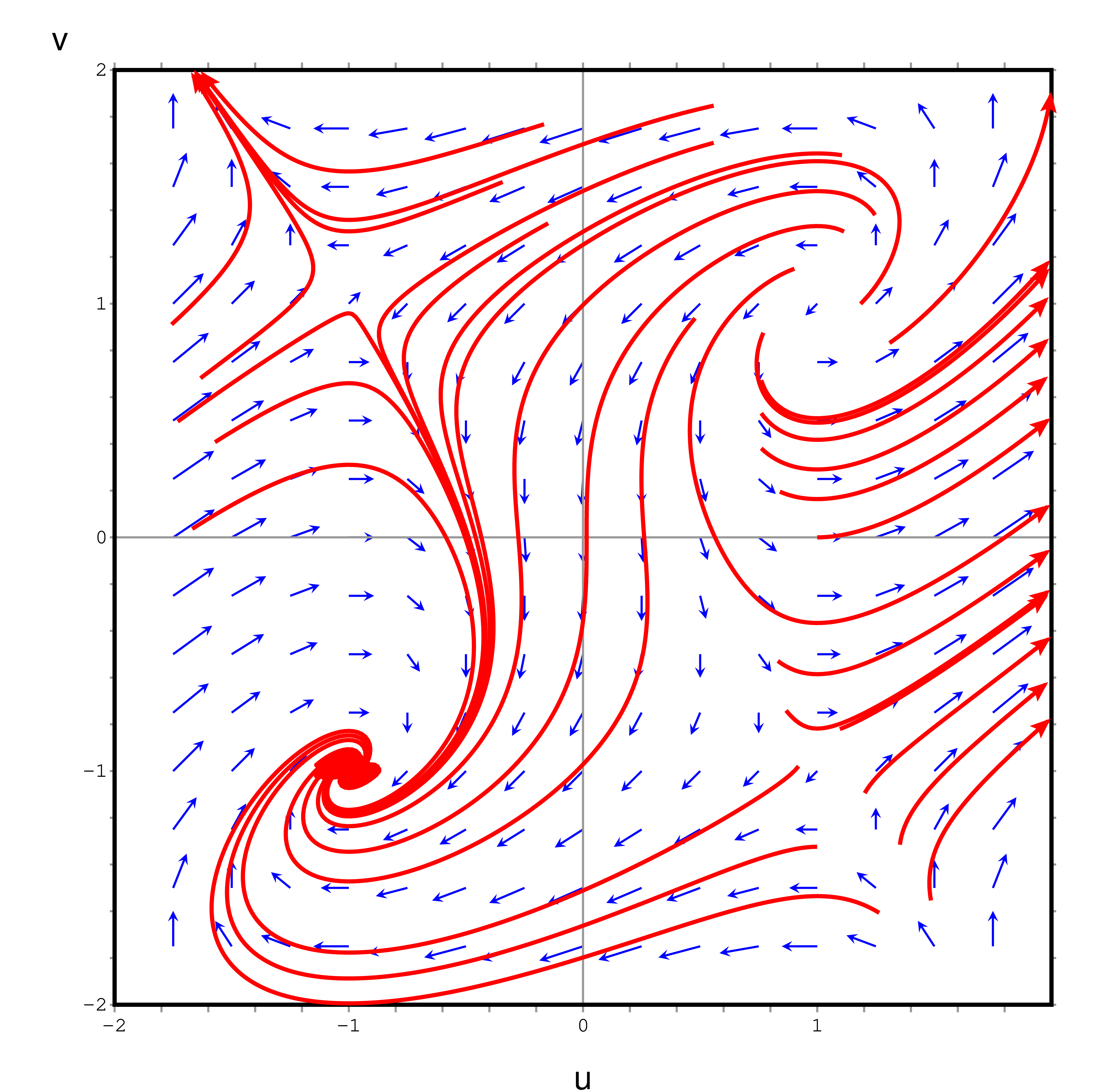1. Is the system linear? Explain why or why not.

2. Identify the equilibrium points of the system.

3. Classify each equilibrium point.

4. Compute the Jacobian $𝑨=\partial 𝑭/\partial 𝒚$ and characterize the eigenvalues of $𝑨$ at each equilibrium point.

Solution.

1. A linear system ${𝒚}^{\text{'}}=𝑨𝒚$, would have equilibrium points $𝑨𝒚=𝟎$. If $𝑨$ is non-singular (linearly independent columns, or non-zero determinant) there would be a single equilibrium. If $𝑨$ is singular, there would be an infinity of solutions, and phase plot would show lines of equilibrium. Since Figure 5 indicates 4 equilibrium points, deduce that system is non-linear.

2. From Figure 5, to within visual precision, the equilibrium points are: $L(1,1),M(-1,1),N(-1,-1),P(1,-1)$.

3. $L$ is an unstable equilibrium point, $N$ is a stable equilibrium point, $M,P$ are saddle points.

4. The Jacobian is

   ${\displaystyle 𝑨=\left(\begin{array}{ll}\frac{\partial f}{\partial u}& \frac{\partial f}{\partial v}\\ \frac{\partial g}{\partial u}& \frac{\partial g}{\partial v}\end{array}\right).}$

   and must have eigenvalues at the equilibrium points of the form:

   L

   ${\lambda }_L=a\pm ib$ with $a>0$ (unstable, spiral trajectories)

   M,P

   ${\lambda }_1,{\lambda }_2$ of different signs (saddle points)

   N

   ${\lambda }_N=c\pm id$, with $c<0$ (stable, spiral trajectories).