Figure 1. PS1.2.2 direction field and solutions
passing through
MATH528Due date: 08/29/18
Follow this model when solving your homework.
8 exercises x .25 = 2 points, 4 problems x .5 = 2 points, 1 project x 1 points = 1 point
Exercise
In[19]:=
ODE = y'[x]==1.5y[x]
In[20]:=
DSolve[ODE,y[x],x]
In[21]:=
Exercise
In[21]:=
ODE = y”[x]==-y[x]
In[22]:=
DSolve[ODE,y[x],x]
In[23]:=
Exercise
In[23]:=
ODE = y'[x]==Cosh[5.13x]
In[24]:=
DSolve[ODE,y[x],x]
In[25]:=
Exercise
In[25]:=
ODE = y”'[x]==Exp[-0.2x]
In[26]:=
DSolve[ODE,y[x],x]
In[27]:=
Exercise
From trigonometric identity , so
In[63]:=
ODE = y'[x]==Sec[y[x]]^2
In[64]:=
DSolve[ODE,y[x],x]
In[65]:=
Integrate[Cos[y]^2,y]
In[66]:=
Exercise
In[67]:=
ODE = y'[x]==Pi y[x] Cos[2Pi x]/Sin[2 Pi x]
In[68]:=
DSolve[ODE,y[x],x]
Exercise
In[69]:=
ODE = y[x] y'[x]+36 x ==0
In[70]:=
DSolve[ODE,y[x],x]
In[71]:=
Exercise
In[69]:=
ODE = y[x] y'[x]+36 x ==0
In[70]:=
DSolve[ODE,y[x],x]
In[71]:=
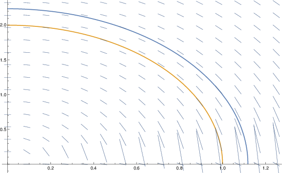
Problem
In[15]:=
f[x_,y_]=-4x/y
In[16]:=
ODE = y'[x]==f[x,y[x]]
In[17]:=
DSolve[ODE,y[x],x]
In[18]:=
From Slide8Lesson01
In[18]:=
Off[DSolve::bvnul];
sol1[x_] = y[x] /. DSolve[{ODE,y[1]==1},y[x],x][[1,1]];
sol2[x_] = y[x] /. DSolve[{ODE,y[0]==2},y[x],x][[1,1]];
{sol1[x],sol2[x]}
In[19]:=
From Slide8Lesson01:
In[20]:=
DirectionField =
VectorPlot[{1,f[x,y]},{x,0,1.25},{y,0,2.5},Axes->True,Frame->False,ImageSize->Large,VectorScale->.3,VectorMarkers->None];
SolutionPlot =
Plot[{sol1[x],sol2[x]},{x,0,1.25},ImageSize->Large];
plots=Show[{SolutionPlot,DirectionField}];
Export["/home/student/courses/MATH528/HW01Fig01.pdf",plots]
In[21]:=
|
Figure 1. PS1.2.2 direction field and solutions
passing through
|
Problem
In[21]:=
f[x_,y_]=1-y^2;
ODE = y'[x]==f[x,y[x]]
In[22]:=
DSolve[ODE,y[x],x]
In[23]:=
Off[Solve::ifun];
sol1[x_] = y[x] /. DSolve[{ODE,y[0]==0},y[x],x][[1,1]];
sol2[x_] = y[x] /. DSolve[{ODE,y[2]==1/2},y[x],x][[1,1]];
{sol1[x],sol2[x]}
In[24]:=
Direction field and solutions
In[24]:=
DirectionField =
VectorPlot[{1,f[x,y]},{x,0,2},{y,-1,1},Axes->True,Frame->False,ImageSize->Large,VectorScale->.051,VectorMarkers->None,VectorStyle->Pink];
SolutionPlot =
Plot[{sol1[x],sol2[x]},{x,0,2},ImageSize->Large];
plots=Show[{SolutionPlot,DirectionField}];
Export["/home/student/courses/MATH528/HW01Fig02.pdf",plots]
In[25]:=
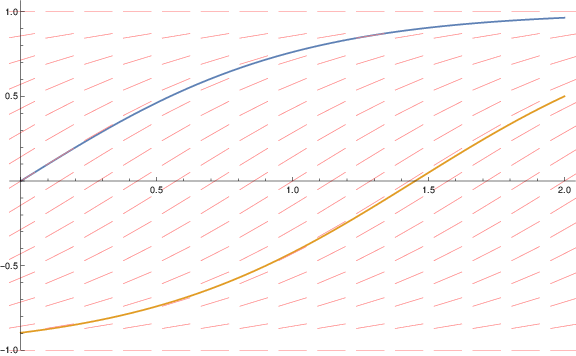 |
Figure 2. PS1.2.2 direction field and solutions
passing through
|
Problem
In[1]:=
ODE = y'[x]^2 - x y'[x] + y[x] == 0
In[5]:=
sol1[x_]=c(x-c)
In[6]:=
Simplify[ODE /. y->sol1]
In[7]:=
sol2[x_]=x^2/4
In[8]:=
Simplify[ODE /. y->sol2]
In[9]:=
DSolve[ODE,y[x],x]
In[10]:=
DSolve[{ODE,y[0]==0},y[x],x]
In[11]:=
Singular solution is the envelope of all particular solutions.
Problem
After 1 day . After 1 year , undetectable since a single atom would weigh
In[11]:=
k=Log[2.]/3.6; y[t_,y0_]=Exp[-k t] y0
In[12]:=
y[1.,1.]
In[13]:=
y[365.25,1.]
In[14]:=
224 1.66 10^(-24)
In[15]:=
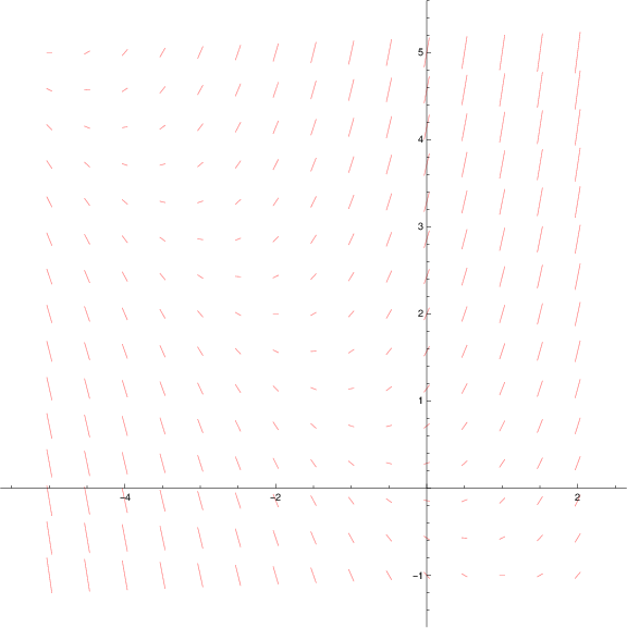
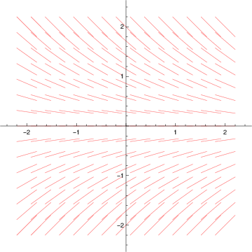
(a) The larger field suggests a pole in quadrant II
In[28]:=
f[x_,y_] = x + y;
DirectionField =
VectorPlot[{1,f[x,y]},{x,-5,2},{y,-1,5},Axes->True,Frame->False,ImageSize->Large,VectorScale->.051,VectorMarkers->None,VectorStyle->Pink];
Export["/home/student/courses/MATH528/HW01Fig03.pdf",DirectionField]
In[29]:=
 |
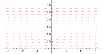
(b) From differentiation by gives
In[35]:=
f[x_,y_] = -x/(9y);
DirectionField =
VectorPlot[{1,f[x,y]},{x,-3,3},{y,0,3},Axes->True,Frame->False,VectorMarkers->None,VectorScale->.051,VectorStyle->Pink,AspectRatio->Automatic];
Export["/home/student/courses/MATH528/HW01Fig04.pdf",DirectionField]
In[36]:=
 |
|
||||||||||||
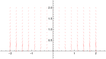
(c) From Table 1, solutions to are circles. Confirm by drawing direction field
In[38]:=
f[x_,y_] = -x/y;
DirectionField =
VectorPlot[{1,f[x,y]},{x,-2,2},{y,0,2},Axes->True,Frame->False,VectorMarkers->None,VectorScale->.1,VectorStyle->Pink,AspectRatio->Automatic];
Export["/home/student/courses/MATH528/HW01Fig05.pdf",DirectionField]
In[39]:=
 |
(d) Solutions to are exponentials. Confirm by drawing direction field
In[39]:=
f[x_,y_] = -y/2;
DirectionField =
VectorPlot[{1,f[x,y]},{x,-2,2},{y,-2,2},Axes->True,Frame->False,VectorMarkers->None,VectorScale->.1,VectorStyle->Pink,AspectRatio->Automatic];
Export["/home/student/courses/MATH528/HW01Fig06.pdf",DirectionField]
In[40]:=
 |