MATH528

MATH528Due date: 09/27/18

Homework 04 - Model solution

1Exercises

Exercise. PS2.2.16

Solution. The basis for $y^{''} + a y^{'} + b y = 0$ is ${e^{r_{1} x}, e^{r_{2} x}}$ with $r_{1, 2}$ distinct roots of the characterisitic equation $r^{2} + a r + b = 0$ , or ${e^{r x}, x e^{r x}}$ for a repeated root. Given roots $r_{1, 2}$ , the characteristic polynomial is $(r - r_{1}) (r - r_{2}) = r^{2} - (r_{1} + r_{2}) r + r_{1} r_{2}$ , hence $a = - (r_{1} + r_{2})$ , $b = r_{1} r_{2}$ . For $r_{1} = 2.6$ , $r_{2} = - 4.3$ , the ODE is

y^{''} + 1.7 y^{'} - 11.18 y = 0 .

Verify:

In[2]:=

ODE = y”[x] + 1.7 y'[x] - 11.18 y[x] == 0;

DSolveValue[ODE,y[x],x]

$c_{1} e^{- 4.3 x} + c_{2} e^{2.6 x}$

In[3]:=

Exercise. PS2.2.17

Solution. Per above, the basis ${e^{- \sqrt{5} x}, x e^{- \sqrt{5} x}}$ indicates $r_{1} = r_{2} = - \sqrt{5}$ is a double root, ${(r + \sqrt{5})}^{2} = r^{2} + 2 \sqrt{5} r + 5 = 0$ , and associated ODE

y^{''} + 2 \sqrt{5} y^{'} + 5 y = 0 .

Verify

In[3]:=

ODE = y”[x] + 2 Sqrt[5] y'[x] + 5 y[x] == 0;

DSolveValue[ODE,y[x],x]

$c_{1} e^{- \sqrt{5} x} + c_{2} e^{- \sqrt{5} x} x$

In[4]:=

Exercise. PS2.2.21

Solution. $y^{''} + 25 y = 0$ has characteristic equation $r^{2}$ +25=0, with roots $r_{1, 2} = \pm 5 i$ , basis ${\cos (5 x), \sin (5 x)}$ , general solution

y = c_{1} \cos (5 x) + c_{2} \sin (5 x), y (0) = c_{1} = 4.6, y^{'} (0) = 5 c_{2} = - 1.2 \Rightarrow c_{1} = 4.6, c_{2} = - . 24 .

Verify

In[4]:=

ODE = y”[x] + 25 y[x] == 0;

DSolveValue[{ODE, y[0]==4.6, y'[0]==-1.2},y[x],x]

$4.6 \cos (5 x) - 0.24 \sin (5 x)$

In[5]:=

Exercise. PS2.2.25

Solution. As, above $y^{''} - y = 0$ , $r^{2} - 1 = 0$ , $y (x) = c_{1} e^{x} + c_{2} e^{- x}$ , $y (0) = c_{1} + c_{2} = 2$ , $y^{'} (0) = c_{1} - c_{2} = - 2$ , $c_{1} = 0$ , $c_{2} = 2$ . Verify:

In[5]:=

ODE = y”[x]- y[x] == 0;

DSolveValue[{ODE,y[0]==2,y'[0]==-2},y[x],x]

$2 e^{- x}$

In[6]:=

Exercise. PS2.8.5

Solution. The ODE $L (y) = (D^{2} + D + 4.25 I) y = 22.1 \cos (4.5 t)$ has solution $y (t) = y_{h} (t) + y_{p} (t)$ with $y_{h} (t) = c_{1} y_{1} (t) + c_{2} y_{2} (t)$ solution of the homogeneous ODE $(D^{2} + D + 4.25 I) y = 0$ with basis ${y_{1} (t), y_{2} (t)}$ , and $y_{p}$ chosen such that $y_{h} + y_{p}$ is a particular solution (i.e., independent of $c_{1}, c_{2}$ )

In[15]:=

L[y_,t_] = D[y[t],{t,2}] + D[y[t],t] + 425/100 y[t]

$y^{''} (t) + y^{'} (t) + \frac{17 y (t)}{4}$

In[16]:=

yh[t_] = DSolveValue[L[y,t]==0,y[t],t]

$c_{1} e^{- t / 2} \sin (2 t) + c_{2} e^{- t / 2} \cos (2 t)$

In[17]:=

From above, the system is damped, hence the steady state $y (t) ≅ y_{p} (t)$ , with $y_{p}$ sought as $y_{p} (t) = a \cos (4.5 t) + b \sin (4.5 t)$ , using method of undetermined coefficients

In[17]:=

yp[t_] = a Cos[45t/10] + b Sin[45t/10]

$a \cos (\frac{9 t}{2}) + b \sin (\frac{9 t}{2})$

In[18]:=

coef = Coefficient[ L[yp,t]-221/10 Cos[45t/10] , {Cos[45t/10],Sin[45t/10]} ]

${- 16 a + \frac{9 b}{2} - \frac{221}{10}, - \frac{9 a}{2} - 16 b}$

In[19]:=

Solve[coef == {0,0},{a,b}]

${{a \to - \frac{32}{25}, b \to \frac{9}{25}}}$

In[20]:=

From above, for large $t$ , $y (t) ≅ [- 32 \cos (9 t / 2) + 9 \sin (9 t / 2)] / 25$ . Verify

In[22]:=

Expand[TrigReduce[DSolveValue[L[y,t]==221/10 Cos[45t/10],y[t],t]]]

$c_{1} e^{- t / 2} \sin (2 t) + c_{2} e^{- t / 2} \cos (2 t) + \frac{9}{25} \sin (\frac{9 t}{2}) - \frac{32}{25} \cos (\frac{9 t}{2})$

In[23]:=

Exercise. PS2.8.7

Solution. As above, for $(4 D^{2} + 12 D + 9 I) y = 225 - 75 \sin (3 t)$

In[1]:=

L[y_,t_] = 4 D[y[t],{t,2}] + 12 D[y[t],t] + 9 y[t]

$4 y^{''} (t) + 12 y^{'} (t) + 9 y (t)$

In[2]:=

yh[t_] = DSolveValue[L[y,t]==0,y[t],t]

$c_{1} e^{- 3 t / 2} + c_{2} e^{- 3 t / 2} t$

In[3]:=

The system is damped with a repeated root. Seek $y_{p} (t) = a \cos (3 t) + b \sin (3 t) + c$

In[3]:=

yp[t_] = a Cos[3t] + b Sin[3t] + c

$a \cos (3 t) + b \sin (3 t) + c$

In[4]:=

coef = Coefficient[ L[yp,t]-(225 -75 Sin[3t]) , {Sin[3t],Cos[3t]} ]

${- 36 a - 27 b + 75, 36 b - 27 a}$

In[5]:=

csol = Solve[coef == {0,0},{a,b}][[1]]

${a \to \frac{4}{3}, b \to 1}$

In[10]:=

Simplify[L[yh,t] + Evaluate[L[yp,t] /. csol] - (225 - 75 Sin[3t])]

$9 (c - 25)$

In[11]:=

From above $y_{p} (t) = \frac{4}{3} \cos (3 t) + \sin (3 t) + 25$ , and the steady state solution is $y (t) ≅ y_{p} (t)$ Verify

In[12]:=

Expand[DSolveValue[L[y,t]==225-75 Sin[3t],y[t],t]]

$c_{1} e^{- 3 t / 2} + c_{2} e^{- 3 t / 2} t + \sin (3 t) + \frac{4}{3} \cos (3 t) + 25$

In[13]:=

Exercise. PS2.8.15

Solution. $(D^{2} + 4 D + 8 I) y = 2 \cos (2 t) + \sin (2 t)$

In[13]:=

L[y_,t_] = D[y[t],{t,2}] + 4 D[y[t],t] + 8 y[t]

$y^{''} (t) + 4 y^{'} (t) + 8 y (t)$

In[14]:=

yh[t_] = DSolveValue[L[y,t]==0,y[t],t]

$c_{1} e^{- 2 t} \sin (2 t) + c_{2} e^{- 2 t} \cos (2 t)$

In[17]:=

Expand[TrigReduce[DSolveValue[L[y,t] == 2 Cos[2t] + Sin[2t],y[t],t]]]

$c_{1} e^{- 2 t} \sin (2 t) + c_{2} e^{- 2 t} \cos (2 t) + \frac{1}{4} \sin (2 t)$

In[18]:=

Exercise. PS2.8.20

Solution. $(D^{2} + 5 I) y = \cos (π t) - \sin (π t)$ , $y (0) = 0$ , $y^{'} (0) = 0$

In[18]:=

L[y_,t_] = D[y[t],{t,2}] + 5 y[t]

$y^{''} (t) + 5 y (t)$

In[19]:=

r[t_] = Cos[Pi t] - Sin[Pi t]

$\cos (π t) - \sin (π t)$

In[23]:=

TrigReduce[DSolveValue[{L[y,t]==r[t],y[0]==0,y'[0]==0},y[t],t]]

$\frac{- \sqrt{5} π \sin (\sqrt{5} t) + 5 \sin (π t) + 5 \cos (\sqrt{5} t) - 5 \cos (π t)}{5 (π^{2} - 5)}$

In[24]:=

2Problems

Problem. PS2.2.31

Solution. ${e^{k x}, x e^{k x}}$ are linearly independent. Proof: from $a e^{k x} + b x e^{k x} = 0$ , obtain $a + b x = 0$ that has to be true for all $x$ , say $x_{1}, x_{2}$ with $x_{1} \neq x_{2}$ leading to a homogeneous system with principal determinant $Δ = x_{2} - x_{1} \neq 0$ , hence only solution is $a = b = 0$ .

Problem. PS2.2.32

Solution. From $c_{1} e^{a x} + c_{2} e^{- a x} = 0$ for $x_{1}, x_{2}$ , $x_{1} \neq x_{2}$ obtain system

𝑨 𝒄 = 𝟎, 𝑨 = (\begin{array}{ll} e^{a x_{1}} & e^{- a x_{1}} \\ e^{a x_{2}} & e^{- a x_{2}} \end{array}), Δ = \det (𝑨) = e^{a (x_{1} - x_{2})} - e^{- a (x_{1} - x_{2})} = z - \frac{1}{z} .

The homogeneous linear system can have a non-zero solution only if $Δ = 0 \Rightarrow z^{2} - 1 = 0 \Rightarrow z = 1 = e^{a (x_{1} - x_{2})} \Rightarrow x_{1} = x_{2}$ contradicting condition $x_{1} = x_{2}$ . Hence $e^{a x}, e^{- a x}$ are linearly independent for all $x$ .

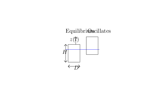
Problem. PS2.4.8

Solution. Sketch defines notation

$z (t)$ is the deviation from equilibrium position
Newton's second law states $m \ddot{z} = F$
Buoy mass is $m = ρ_{b} \frac{π}{4} D^{2} H$
$g$ is gravitational acceleration
Force imbalance when buoy is out of equilibrium is $F = - ρ_{b}$ $\frac{π}{4} D^{2} z g$
Buoy oscilations described by
$\ddot{z} + \frac{g}{H} z = 0$
with solution
$z (t) = a \cos (ω t), ω = \frac{2 π}{T} = \sqrt{\frac{g}{H}} \Rightarrow H = g {(\frac{T}{2 π})}^{2} = \frac{10}{π^{2}} ≅ 1 m .$

Problem. PS2.4.14

Solution. The car suspension dynamics is described by

m \ddot{z} + c \dot{z} + k z = 0,

with $c$ given by the critical damping condition $c = \sqrt{4 m k} = \sqrt{4 \times 2000 \times 4500} = 6000 \sec^{- 1}$

3Projects

3.1PS2.8.24

The gun barrel is modeled as $y^{''} + y = r (t)$ , $y (0) = 0$ , $y^{'} (0) = 0$ , with

r (t) = {\begin{cases} 1 - {(t / π)}^{2} & for 0 ⩽ t ⩽ π \\ 0 & for t > π \end{cases} . .

In[28]:=

L[y_,t_] = D[y[t],{t,2}] + y[t]

$y^{''} (t) + y (t)$

In[29]:=

r[t_]=1-(t/Pi)^2

$1 - \frac{t^{2}}{π^{2}}$

In[30]:=

Solve the IVP to find motion up to $t = π$

In[32]:=

sol1[t_]=DSolveValue[{L[y,t]==r[t],y[0]==0,y'[0]==0},y[t],t]

$\frac{- t^{2} - π^{2} \cos (t) - 2 \cos (t) + π^{2} + 2}{π^{2}}$

In[33]:=

Find position, velocity at $t = π$

In[33]:=

u={sol1[Pi],sol1'[t] /. t->Pi}

${\frac{4 + π^{2}}{π^{2}}, - \frac{2}{π}}$

In[34]:=

Now solve the homogeneous ODE for $t > π$

In[38]:=

sol2[t_]=DSolveValue[Flatten[{L[y,t]==0,{y[Pi],y'[Pi]}==u}],y[t],t]

$\frac{2 π \sin (t) - π^{2} \cos (t) - 4 \cos (t)}{π^{2}}$

In[39]:=

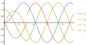
Define the full solution along with some interesting derivatives and plot it

In[43]:=

sol[t_]:=If[t<=Pi,sol1[t],sol2[t]];

plt = Plot[{sol[t],sol'[t],sol”[t],sol”'[t]},{t,0,3Pi},PlotLegends->Automatic];

Export["/home/student/courses/MATH528/HW04Fig01.pdf",plt]

$/home/student/courses/MATH528/HW04Fig01.pdf$

In[44]:=

The plot is rendered in Fig. 1

Figure 1.