MATH528

MATH52809/28/18

Mini-Lab 05

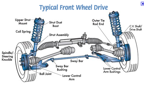
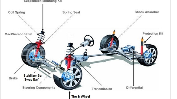
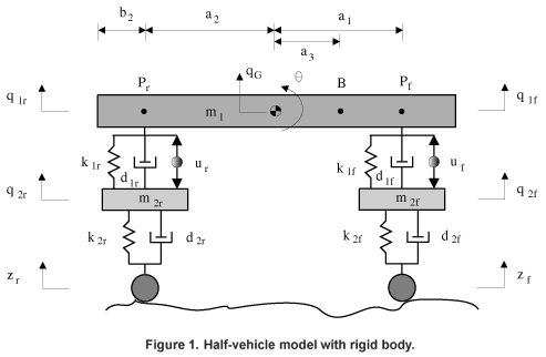
In a two-mini-lab sequence, we study a realistic model: the dynamics of a car. In this first mini-lab we solve some simpler lead-up problems involving point masses and springs

Terrain modeled by known functions $z_{f} (t), z_{r} (t)$
Car suspension described by: $q_{1 f} (t), q_{2 f} (t), q_{1 r} (t), q_{2 r} (t)$
Dynamics described by Newton's law for linear and angular momentum

\begin{array}{rcl} m_{2 r} {\ddot{q}}_{2 r} & = & k_{1 r} (q_{1 r} - q_{2 r}) - k_{2 r} (q_{2 r} - z_{r}) + d_{1 r} ({\dot{q}}_{1 r} - {\dot{q}}_{2 r}) - d_{2 r} ({\dot{q}}_{2 r} - {\dot{z}}_{r}) \\ m_{2 f} {\ddot{q}}_{2 f} & = & k_{1 f} (q_{1 f} - q_{2 f}) - k_{2 f} (q_{2 f} - z_{f}) + d_{1 f} ({\dot{q}}_{1 f} - {\dot{q}}_{2 f}) - d_{2 f} ({\dot{q}}_{2 f} - {\dot{z}}_{f}) \\ m_{1} \frac{{\ddot{q}}_{1 r} + {\ddot{q}}_{1 f}}{2} & = & - k_{1 r} (q_{1 r} - q_{2 r}) - k_{1 f} (q_{1 f} - q_{2 f}) - d_{1 r} ({\dot{q}}_{1 r} - {\dot{q}}_{2 r}) - d_{1 f} ({\dot{q}}_{1 f} - {\dot{q}}_{2 f}) \\ I \frac{{\ddot{q}}_{1 f} - {\ddot{q}}_{1 r}}{2 a} & = & a [k_{1 r} (q_{1 r} - q_{2 r}) + d_{1 r} ({\dot{q}}_{1 r} - {\dot{q}}_{2 r})] - a [k_{1 f} (q_{1 f} - q_{2 f}) + d_{1 f} ({\dot{q}}_{1 f} - {\dot{q}}_{2 f})] \end{array}

1Warm-up problems: lossless oscillators in series

1.1Single spring

Figure 1. Two springs connected in series

Consider the model resulting from conservation of momentum

\begin{array}{rcl} \dot{u_{1}} & = & - \frac{k_{1}}{m_{1}} x_{1} \\ {\dot{x}}_{1} & = & u_{1} \end{array}

that can expressed in vector form as

𝒚^{'} = 𝑨 𝒚 + 𝒇, 𝒚 = (\begin{array}{l} u_{1} \\ x_{1} \end{array}), 𝑨 = (\begin{array}{ll} 0 & - \frac{k_{1}}{m_{1}} \\ 1 & 0 \end{array}), 𝒇 = (\begin{array}{l} f_{1} \\ 0 \end{array})

Define the system matrix in Mathematica

In[1]:=

A={{0,-k1/m1},{1,0}};

MatrixForm[A]

$(\begin{array}{cc} 0 & - \frac{k1}{m1} \\ 1 & 0 \end{array})$

In[2]:=

Define the number of components in the dependent variable $𝒚 (t)$ and the forcing term $f$

In[2]:=

y[t_]={y1[t],y2[t]};

f[t_]={f1[t],0};

SYS = y'[t] == A . y[t] + f[t];

MatrixForm[A . y[t] + f[t]]

$(\begin{array}{c} f1 (t) - \frac{k1y2 (t)}{m1} \\ y1 (t) \end{array})$

In[3]:=

Now, look at the solutions for some typical initial conditions and forcing terms:

Case 1

No initial velocity, point masses out of equilibrium position, no forcing. Define a set of replacement rules for the system parameters defining this case

In[3]:=

F1[t_]=0;

case1 = {f1->F1,m1->1,k1->1}

${f1 \to F1, m1 \to 1, k1 \to 1}$

In[4]:=

The system matrix for this case:

In[4]:=

MatrixForm[A /. case1]

$(\begin{array}{cc} 0 & - 1 \\ 1 & 0 \end{array})$

In[5]:=

Find the eigenvalues

In[5]:=

MatrixForm[DiagonalMatrix[Eigenvalues[A /. case1]]]

$(\begin{array}{cc} i & 0 \\ 0 & - i \end{array})$

In[6]:=

MatrixForm[Eigenvectors[A /. case1]]

$(\begin{array}{cc} i & 1 \\ - i & 1 \end{array})$

In[7]:=

As expected, eigenvalues are purely imaginary indicating oscillations with no dampening. Solve the system for some chosen set of initial conditions

In[7]:=

iCond = {0,1};

F1[t_]=0;

MatrixForm[SYS /. case1]

${{y1}^{'} (t), {y2}^{'} (t)} = {- y2 (t), y1 (t)}$

In[8]:=

GenSol[t_] = DSolveValue[ SYS /. case1, y[t],t]

${c_{1} \cos (t) - c_{2} \sin (t), c_{1} \sin (t) + c_{2} \cos (t)}$

In[9]:=

c={C[1],C[2]};

sol[t_] = GenSol[t] /. Solve[GenSol[0] == iCond,c]

$(\begin{array}{cc} - \sin (t) & \cos (t) \end{array})$

In[11]:=

SingleOscPlt1 = ParametricPlot[sol[t],{t,0,2Pi},Axes->True,Frame->True,FrameLabel->{"y1","y2"}];

Export["/home/student/courses/MATH528/L05Fig01.pdf",SingleOscPlt1]

$/home/student/courses/MATH528/L05Fig01.pdf$

In[12]:=

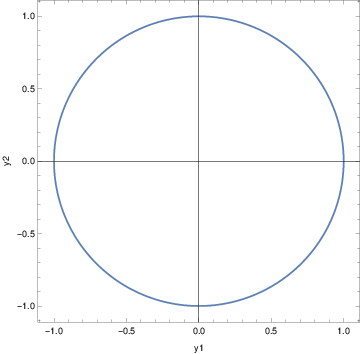Figure 2. Phase plane trajectory for unforced harmonic oscillator

Case 2

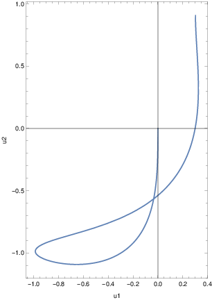
No initial velocity, point masses at equilibrium, with forcing

In[12]:=

F1[t]=Sin[2t];

case2 = {f1->F1,m1->1,k1->1};

GenSol[t_] = DSolveValue[ SYS /. case1, y[t],t]

${- c_{2} \sin (t) + c_{1} \cos (t) + \frac{2 \sin^{4} (t)}{3} + \cos (t) (- \frac{\cos (t)}{2} - \frac{1}{6} \cos (3 t)), c_{1} \sin (t) + c_{2} \cos (t) - \frac{2}{3} \sin^{3} (t) \cos (t) + \sin (t) (- \frac{\cos (t)}{2} - \frac{1}{6} \cos (3 t))}$

In[17]:=

c={C[1],C[2]};

sol[t_] = TrigReduce[GenSol[t] /. Solve[GenSol[0] == iCond,c]]

$(\begin{array}{cc} \frac{1}{3} (2 \cos (t) - 2 \cos (2 t) - 3 \sin (t)) & \frac{1}{3} (3 \cos (t) + 2 \sin (t) - \sin (2 t)) \end{array})$

In[18]:=

SingleOscPlt2 = ParametricPlot[sol[t],{t,0,2Pi},Axes->True,Frame->True,FrameLabel->{"y1","y2"}];

Export["/home/student/courses/MATH528/L05Fig02.pdf",SingleOscPlt2]

$/home/student/courses/MATH528/L05Fig02.pdf$

In[19]:=

Figure 3. Phase trajectory for forced oscillator

1.2Two springs in series

Figure 4. Two springs connected in series

Consider the model resulting from conservation of momentum

\begin{array}{rcl} {\dot{x}}_{1} & = & u_{1} \\ \dot{x_{2}} & = & u_{2} \\ \dot{u_{1}} & = & - \frac{k_{1}}{m_{1}} x_{1} + \frac{k_{2}}{m_{1}} (x_{2} - x_{1}) + f_{1} \\ \dot{u_{2}} & = & - \frac{k_{2}}{m_{2}} (x_{2} - x_{1}) + f_{2} \end{array}

that can expressed in vector form as

𝒚^{'} = 𝑨 𝒚 + 𝒇, 𝒚 = (\begin{array}{l} u_{1} \\ u_{2} \\ x_{1} \\ x_{2} \end{array}), 𝑨 = (\begin{array}{llll} 0 & 0 & - \frac{k_{1} + k_{2}}{m_{1}} & \frac{k_{2}}{m_{1}} \\ 0 & 0 & - \frac{k_{2}}{m_{2}} & - \frac{k_{2}}{m_{2}} \\ 1 & 0 & 0 & 0 \\ 0 & 1 & 0 & 0 \end{array}), 𝒇 = (\begin{array}{l} f_{1} \\ f_{2} \\ 0 \\ 0 \end{array})

Define the system matrix in Mathematica

In[1]:=

A={{0,0,-(k1+k2)/m1,k2/m1},{0,0,k2/m2,-k2/m2},{1,0,0,0},{0,1,0,0}};

MatrixForm[A]

$(\begin{array}{cccc} 0 & 0 & - \frac{k1 + k2}{m1} & \frac{k2}{m1} \\ 0 & 0 & \frac{k2}{m2} & - \frac{k2}{m2} \\ 1 & 0 & 0 & 0 \\ 0 & 1 & 0 & 0 \end{array})$

In[2]:=

Define the number of components in the dependent variable $𝒚 (t)$ and the forcing term $f$

In[2]:=

y[t_]={y1[t],y2[t],y3[t],y4[t]};

f[t_]={f1[t],f2[t],0,0};

SYS = y'[t] == A . y[t] + f[t];

MatrixForm[A . y[t] + f[t]]

$(\begin{array}{c} f1 (t) - \frac{(k1 + k2) y3 (t)}{m1} + \frac{k2y4 (t)}{m1} \\ f2 (t) + \frac{k2y3 (t)}{m2} - \frac{k2y4 (t)}{m2} \\ y1 (t) \\ y2 (t) \end{array})$

In[3]:=

Now, look at the solutions for some typical initial conditions and forcing terms:

Case 1

No initial velocity, point masses out of equilibrium position, no forcing. Define a set of replacement rules for the system parameters defining this case

In[3]:=

case1 = {f1->F1,f2->F2,m1->1,m2->1,k1->1,k2->1}

${f1 \to F1, f2 \to F2, m1 \to 1, m2 \to 1, k1 \to 1, k2 \to 1}$

In[4]:=

The system matrix for this case:

In[4]:=

MatrixForm[A /. case1]

$(\begin{array}{cccc} 0 & 0 & - 2 & 1 \\ 0 & 0 & 1 & - 1 \\ 1 & 0 & 0 & 0 \\ 0 & 1 & 0 & 0 \end{array})$

In[5]:=

Find the eigenvalues

In[5]:=

MatrixForm[DiagonalMatrix[Eigenvalues[A /. case1]]]

$(\begin{array}{cccc} i \sqrt{\frac{1}{2} (3 + \sqrt{5})} & 0 & 0 & 0 \\ 0 & - i \sqrt{\frac{1}{2} (3 + \sqrt{5})} & 0 & 0 \\ 0 & 0 & i \sqrt{\frac{1}{2} (3 - \sqrt{5})} & 0 \\ 0 & 0 & 0 & - i \sqrt{\frac{1}{2} (3 - \sqrt{5})} \end{array})$

In[6]:=

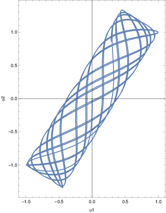
As expected, eigenvalues are purely imaginary indicating oscillations with no dampening. Solve the system for some chosen set of initial conditions. As the system matrix size increases analytical expressions for the eigenvalues, eigenvectors become complicated or impossible to find.

In[8]:=

iCond = {0,0,1,2};

{F1[t_],F2[t_]}={0,0};

MatrixForm[A . y[t] + f[t] /. case1]

$(\begin{array}{c} y4 (t) - 2 y3 (t) \\ y3 (t) - y4 (t) \\ y1 (t) \\ y2 (t) \end{array})$

In[9]:=

We turn to numerical evaluation of the solution to the system of ODEs

In[20]:=

sol[t_]=NDSolveValue[ {y'[t]==A . y[t] + f[t] /. case1,y[0]==iCond}, y[t],{t,0,32Pi}];

DoubleOscPlt1 = ParametricPlot[sol[t][[1;;2]],{t,0,32Pi},Axes->True,Frame->True,FrameLabel->{"u1","u2"}];

Export["/home/student/courses/MATH528/L05Fig03.pdf",DoubleOscPlt1]

$/home/student/courses/MATH528/L05Fig03.pdf$

In[21]:=

Figure 5. Phase plane of velocities of the double spring