1.Quantities

1.1.Numbers

Most scientific disciplines introduce an idea of the amount of some entity or property of interest. Furthermore, the amount is usually combined with the concept of a number, an abstraction of the observation that the two sets $A=${Mary, Jane, Tom} and $B=${apple, plum, cherry} seem quite different, but we can match one distinct person to one distinct fruit as in {Mary$\to$plum, Jane$\to$apple, Tom$\to$cherry}. In contrast we cannot do the same matching of distinct persons to a distinct color from the set {red, green}, and one of the colors must be shared between two persons. Formal definition of the concept of a number from the above observations is surprisingly difficult since it would be self-referential due to the apperance of the numbers “one” and “two”. Leaving this aside, the key concept is that of quantity of some property of interest that is expressed through a number. Several types of numbers have been introduced in mathematics to express different types of quantities, and the following will be used throughout this text:

$\mathbb{N}$

The set of natural numbers, $\mathbb{N}=\{0,1,2,3,\dots \}$, infinite and countable, ${\mathbb{N}}_{+}=\{1,2,3,\dots \}$;

$\mathbb{Z}$

The set of integers, $\mathbb{Z}=\{0,\pm 1,\pm 2,\pm 3,\dots \}$, infinite and countable;

$\mathbb{Q}$

The set of rational numbers $\mathbb{Q}=\{p/q,p\in \mathbb{Z},q\in {\mathbb{N}}_{+}\}$, infinite and countable;

$ℝ$

The set of real numbers, infinite, not countable, can be ordered;

$ℂ$

The set of complex numbers, $ℂ=\{x+iy,x,y\in ℝ\}$, infinite, not countable, cannot be ordered.

A computer has a finite amount of memory, hence cannot represent all numbers, but rather subsets of the above sets. Furthermore, computers internally use binary numbers composed of binary digits, or bits. Many computer number types are defined for specific purposes, and are often encountered in applications such as image representation or digital data acquisition. Here are the main types.

Subsets of $\mathbb{N}$

The number types uint8, uint16, uint32, uint64 represent subsets of the natural numbers (unsigned integers) using 8, 16, 32, 64 bits respectively. An unsigned integer with $b$ bits can store a natural number in the range from $0$ to $2^b-1$. Two arbitrary natural numbers, written as $\forall i,j\in \mathbb{N}$ can be added and will give another natural number, $k=i+j\in \mathbb{N}$. In contrast, addition of computer unsigned integers is only defined within the specific range $0$ to $2^b-1$.

octave]

i=uint8(15); j=uint8(10); k=i+j

k = 25

octave]

i=uint8(150); j=uint8(200); k=i+j

k = 255

octave]

k=i-j

k = 0

octave]

Subsets of $\mathbb{Z}$

The number types int8, int16, int32, int64 represent subsets of the integers. One bit is used to store the sign of the number, so the subset of $\mathbb{Z}$ that can be represented is from $1-2^{b-1}$ to $2^{b-1}-1$

octave]

i=int8(100); j=int8(101); k=i+j

k = 127

octave]

k=i-j

k = -1

octave]

Subsets of $\mathbb{Q},ℝ,ℂ$

Computers approximate the real numbers through the set $𝔽$ of floating point numbers. Floating point numbers that use $b=32$ bits are known as single precision, while those that use $b=64$ are double precision. A floating point number $x\in 𝔽$ is stored internally as $x=\pm .B_1{B}_2\dots B_m\times 2^{\pm b_1{b}_2\dots b_e}$ where $B_i$, $i=1,\dots ,m$are bits within the mantissa of length $m$, and $b_j$, $j=1,\dots ,e$ are bits within the exponent, along with signs $\pm$ for each. The default number type is usually double precision, more concisely referred to double. Common constants such as $e$, $\pi$ are predefined as double, can be truncated to single, and the number of displayed decimal digits is controlled by format. The function disp(x) displays its argument x.

octave]

format long; disp([e pi])

2.718281828459045 3.141592653589793

octave]

disp([single(e) single(pi)])

2.7182817 3.1415927

octave]

The approximation of the reals $ℝ$ by the floats $𝔽$ is characterized by: realmax, the largest float, realmin the smallest positive float, and eps known as machine epsilon. Machine epsilon highlights the differences between floating point and real numbers since it is defined as the largest number $ϵ\in 𝔽$ that satisfies $1+ϵ=1$. If $\epsilon \in ℝ$ of course $1+\epsilon =1$ implies $\epsilon =0$, but floating points exhibit “granularity”, in the sense that over a unit interval there are small steps that are indistinguishable from zero due to the finite number of bits available for a float. Machine epsilon is small, and floating point errors can usually be kept under control. Keep in mind that perfect accuracy is a mathematical abstraction, not encountered in nature. In fields as sociology or psychology 3 digits of accuracy are excellent, in mechanical engineering this might increase to 6 digits, or in electronic engineering to 8 digits. The most precisely known physical constant is the Rydberg constant known to 12 digits. The granularity of double precision expressed by machine epsilon is sufficient to represent natural phenomena.

octave]

format short; disp([realmin realmax eps 1+eps])

2.2251e-308 1.7977e+308 2.2204e-16 1.0000e+00

octave]

Within the reals certain operations are undefined such as $1/0$. Special float constants are defined to handle such situations: Inf is a float meant to represent infinity, and NaN (“not a number”) is meant to represent an undefinable result of an arithmetic operation.

octave]

warning("off"); disp([Inf 1/0 2*realmax NaN Inf-Inf Inf/Inf])

Inf Inf Inf NaN NaN NaN

octave]

Complex numbers $z\in ℂ$ are specified by two reals, in Cartesian form as $z=x+iy$, $x,y\in ℝ$ or in polar form as $z=\rho e^{i\theta }$, $\rho ,\theta \in ℝ$, $\rho ⩾0$. The computer type complex is similarly defined from two floats and the additional constant I is defined to represent $\sqrt{-1}=i=e^{i\pi /2}$. Functions are available to obtain the real and imaginary parts within the Cartesian form, or the absolute value and argument of the polar form.

octave]

z1=complex(1,1); z2=complex(1,-1); disp([z1+z2 z1/z2])

2 + 0i 0 + 1i

octave]

disp([real(z1) real(z2) real(z1+z2) real(z1/z2)])

1 1 2 0

octave]

disp([imag(z1) imag(z2) imag(z1+z2) imag(z1/z2)])

1 -1 0 1

octave]

disp([abs(z1) abs(z2) abs(z1+z2) abs(z1/z2)])

1.4142 1.4142 2.0000 1.0000

octave]

disp([arg(z1) arg(z2) arg(z1+z2) arg(z1/z2)])

0.78540 -0.78540 0.00000 1.57080

octave]

I-sqrt(-1)

ans = 0

octave]

Care should be exercised about the cummulative effect of many floating point errors. For instance, in an “irrational” numerical investigation of Zeno's paradox, one might want to compare the distance $S_N$ traversed by step sizes that are scaled by $1/\pi$ starting from one to $T_N$, traversed by step sizes scaled by $\pi$ starting from ${\pi }^{-N}$

In the reals the above two expressions are equal, $S_N=T_N$, but this is not verfied for all $N$ when using floating point numbers. Lists of the values ${\pi }^j$, for the two orderings $j=0,\dots ,N$, and $j=N,\dots ,0$, can be generated and summed.

octave] 

N=10; S=pi.^(0:-1:-N); T=pi.^(-N:1:0); sum(S)==sum(T)

octave] 

N=15; S=pi.^(0:-1:-N); T=pi.^(-N:1:0); sum(S)==sum(T)

octave] 

In the above numerical experiment a==b expresses an equality relationship which might evaluate as true denoted by 1, or false denoted by 0.

octave] 

disp([1==1 1==2])

octave] 

The above was called an “irrational” investigation since in Zeno's original paradox the scaling factor was 2 rather than $\pi$, and due to the binary representation used by floats equality always holds.

octave] 

N=30; S=2.^(0:-1:-N); T=2.^(-N:1:0); sum(S)==sum(T)

octave] 

1.2.Quantities described by a single number

The above numbers and their computer approximations are sufficient to describe many quantities encountered in applications. Typical examples include:

• the position $x\in ℝ$ of a point on the unit line segment $[0,1]$, approximated by the floating point number $\stackrel{\sim }{x}\in 𝔽$, to within machine epsilon precision, $|x-\stackrel{\sim }{x}|⩽ϵ$;

• the measure of resistance to change of the rate of motion known as mass, $m\in ℝ$, $m>0$;

• the population of a large community expressed as a float $p\in 𝔽$, even though for a community of individuals the population is a natural number, as in “the population of the United States is $p=328.2\text{E6}$, i.e., 328.2 million”.

In most disciplines, there is a particular interest in comparison of two quantities, and to facilitate such comparison a common reference is used known as a standard unit. For measurement of a length $L$, the meter $\ell =1\text{m}$ is a standard unit, as in the statement $L=10\text{m}$, that states that $L$ is obtained by taking the standard unit ten times, $L=10\ell$. The rules for carrying out such comparisons are part of the definition of real and rational numbers. These rules are formalized in the mathematical definition of a field $(F,+,\times )$ presented in the next chapter. Quantities that obey such rules, i.e., belong to a field, can be used in changes of scale and are called scalars. Not all numbers are scalars in this sense. For instance, the integers would not allow a scaling of 1:2 (halving the scale) even though 1,2 are integers.

1.3.Quantities described by multiple numbers

Other quantities require more than a single number. The distribution of population in the year 2000 among the alphabetically-ordered South American countries (Argentina, Bolivia,..,Venezuela) requires 12 numbers. These are placed together in a list known in mathematics as a tuple, in this case a 12-tuple $P=(p_1,p_2,\dots ,p_{12})$, with $p_1$ the population of Argentina, $p_2$ that of Bolivia, and so on. An analogous 12-tuple can be formed from the South American populations in the year 2020, say $Q=(q_1,q_2,\dots ,q_{12})$. Note that it is difficult to ascribe meaning to apparently plausible expressions such as $P+Q$ since, for instance, some people in the 2000 population are also in the 2020 population, and would be counted twice.

2.Vectors

2.1.Vector spaces

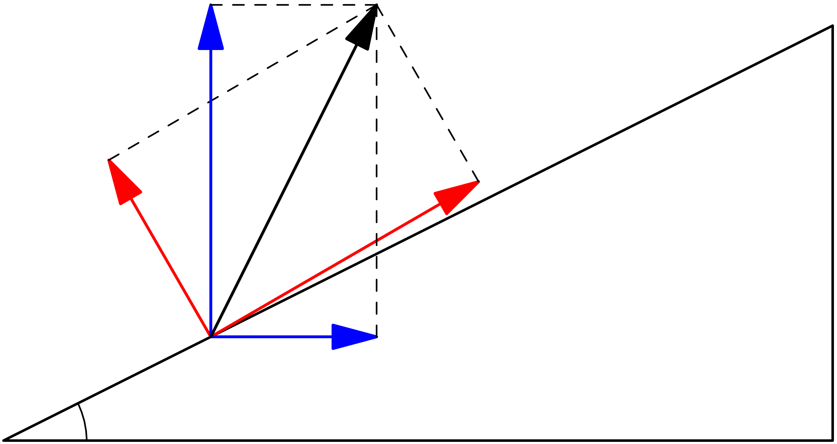
In contrast to the population 12-tuple example above, combining multiple numbers is well defined in operations such as specifying a position within a three-dimensional Cartesian grid, or determining the resultant of two forces in space. Both of these lead to the consideration of 3-tuples or triples such as the force $(f_1,f_2,f_3)$. When combined with another force $(g_1,g_2,g_3)$ the resultant is $(f_1+g_1,f_2+g_2,f_3+g_3)$. If the force $(f_1,f_2,f_3)$ is amplified by the scalar $\alpha$ and the force $(g_1,g_2,g_3)$ is similarly scaled by $\beta$, the resultant becomes

It is useful to distinguish tuples for which scaling and addition is well defined from simple lists of numbers. In fact, since the essential difference is the behavior with respect to scaling and addition, the focus should be on these operations rather than the elements of the tuple.

The above observations underlie the definition of a vector space $𝒱$ by a set $V$ whose elements satisfy certain scaling and addition properties, denoted all together by the 4-tuple $𝒱=(V,S,+,\cdot )$. The first element of the 4-tuple is a set whose elements are called vectors. The second element is a set of scalars, and the third is the vector addition operation. The last is the scaling operation, seen as multiplication of a vector by a scalar. The vector addition and scaling operations must satisfy rules suggested by positions or forces in three-dimensional space, which are listed in Table 1. In particular, a vector space requires definition of two distinguished elements: the zero vector $𝟎\in V$, and the identity scalar element $1\in S$.

The definition of a vector space reflects everyday experience with vectors in Euclidean geometry, and it is common to refer to such vectors by descriptions in a Cartesian coordinate system. For example, a position vector $𝒓$ within the plane can be referred through the pair of coordinates $(x,y)$. This intuitive understanding can be made precise through the definition of a vector space ${ℛ}_2=({ℝ}^2,ℝ,+,\cdot )$, called the real 2-space. Vectors within ${ℛ}_2$ are elements of ${ℝ}^2=ℝ\times ℝ=\{(x,y)|.x,y\in ℝ\}$, meaning that a vector is specified through two real numbers, $𝒓\leftrightarrow (x,y)$. Addition of two vectors, $𝒒\leftrightarrow (s,t)$, $𝒓\leftrightarrow (x,y)$ is defined by addition of coordinates $𝒒+𝒓=(s+x,t+v)$. Scaling $𝒓\leftrightarrow (x,y)$ by scalar $a$ is defined by $a𝒓\leftrightarrow (ax,ay)$. Similarly, consideration of position vectors in three-dimensional space leads to the definition of the ${ℛ}_3=({ℝ}^3,ℝ,+,\cdot )$, or more generally a real $m$-space ${ℛ}_m=({ℝ}^m,ℝ,+,\cdot )$, $m\in \mathbb{N}$, $m>0$.

Note however that there is no mention of coordinates in the definition of a vector space as can be seen from the list of properties in Table 1. The intent of such a definition is to highlight that besides position vectors, many other mathematical objects follow the same rules. As an example, consider the set of all continuous functions $C\left(ℝ\right)=\{f|.f:ℝ\to ℝ\}$, with function addition defined by the sum at each argument $t,$ $(f+g)\left(t\right)=f\left(t\right)+g\left(t\right)$, and scaling by $a\in ℝ$ defined as $(af)\left(t\right)=af\left(t\right)$. Read this as: “given two continuous functions $f$ and $g$, the function $f+g$ is defined by stating that its value for argument $x$ is the sum of the two real numbers $f\left(t\right)$ and $g\left(t\right)$”. Similarly: “given a continuous function $f$, the function $af$ is defined by stating that its value for argument $t$ is the product of the real numbers $a$ and $f\left(t\right)$”. Under such definitions ${𝒞}^0=(C\left(ℝ\right),ℝ,+,\cdot )$ is a vector space, but quite different from ${ℛ}_m$. Nonetheless, the fact that both ${𝒞}^0$ and ${ℛ}_m$ are vector spaces can be used to obtain insight into the behavior of continuous functions from Euclidean vectors, and vice versa.

2.2.Real vector space ${ℛ}_m$

Column vectors.

with the components arranged vertically and enclosed in square brackets. Given two vectors $𝒖,𝒗\in {ℝ}^m$, and a scalar $a\in ℝ$, vector addition and scaling are defined in ${ℛ}_m$ by real number addition and multiplication of components

The vector space ${ℛ}_m$ is defined using the real numbers as the set of scalars, and constructing vectors by grouping together $m$ scalars, but this approach can be extended to any set of scalars $S$, leading to the definition of the vector spaces ${𝒮}_n=(S^n,S,+,\cdot )$. These will often be referred to as $n$-vector space of scalars, signifying that the set of vectors is $V=S^n$.

To aid in visual recognition of vectors, the following notation conventions are introduced:

vectors are denoted by lower-case bold Latin letters: $𝒖,𝒗$;

scalars are denoted by normal face Latin or Greek letters: $a,b,\alpha ,\beta$;

the components of a vector are denoted by the corresponding normal face with subscripts as in equation (1);

related sets of vectors are denoted by indexed bold Latin letters: ${𝒖}_1,{𝒖}_2,\dots ,{𝒖}_n$.

In Octave, successive components placed vertically are separated by a semicolon.

octave] 

[1; 2; -1; 2]

octave] 

The equal sign in mathematics signifies a particular equivalence relationship. In computer systems such as Octave the equal sign has the different meaning of assignment, that is defining the label on the left side of the equal sign to be the expression on the right side. Subsequent invocation of the label returns the assigned object. Components of a vector are obtained by enclosing the index in parantheses.

octave] 

u=[1; 2; -1; 2]; u

octave] 

u(3)

octave] 

Row vectors.

and ${𝒖}^T$ is the notation used to denote a row vector. In Octave, horizontal placement of successive components in a row is denoted by a space.

octave] 

uT=transpose(u)

octave] 

[1 2 -1 2]

octave] 

uT(4)

octave] 

Compatible vectors.

octave] 

uT=[1 0 1 2]; vT=[2 1 3 -1]; wT=uT+vT; disp(wT)

octave] 

rT=[1 2]; uT+rT

octave] 

a=3; zT=a*uT; disp(zT)

octave] 

2.3.Working with vectors

Ranges.

octave] 

m=4; disp(1:m)

octave] 

disp(m:-1:2)

octave] 

r=0; s=0.2; t=1; disp(r:s:t)

octave] 

r=0; s=0.3; t=1; disp(r:s:t)

octave] 

r=0; s= -0.2; t=1; disp(r:s:t)

octave] 

An efficient, expressive feature of many software systems including Octave is to use ranges as indices to a vector, as shown below for the definition of $𝟎\in {ℝ}^4$. Note that the index range i is organized as a row, and a transpose operation must be applied to obtain z as a column vector.

octave] 

m=4; i=1:m; z(i)=i.^i; z=transpose(z); disp(z)

octave] 

i

octave] 

disp(transpose(z))

octave] 

Visualization.

octave] 

 t=0:0.1:1.5; disp(sin(t))

octave] 

Indeed, such a piece-by-piece approach is not the way humans organize large amounts of information, preferring to conceptualize the data as some other entity: an image, a sound excerpt, a smell, a taste, a touch, a sense of balance, or relative position. All seven of these human senses will be shown to allow representation by linear algebra concepts, including representation by vectors.

As a first example consider visualization, the process of transforming data into a sight perception. A familiar example is constructing a plot of the graph of a function. Recall that in mathematics the graph of a function $f:X\to Y$ relating elements of the domain $X$ to those in codomain $Y$ is a set of ordered pairs $G_f=\left\{(x,y)|y=f\left(x\right),x\in X.\right\}$. For a commonly encountered function such as $\sin :[0,2\pi )\to [-1,1]$, the graph $G_{\sin }=\{(x,\sin \left(x\right))|x\in [0,2\pi .)\}$ contains an uncountably infinite number of elements, and obviously cannot be explicitly listed. The sine function is continuous, meaning that no matter how small an open interval $(c,d)$ within the function codomain $[-1,1]$ one considers, there exists an interval $(a,b)$ in the function domain $[0,2\pi ]$ whose image by the sine function is contained in $(c,d)$. In mathematical “$\delta -\epsilon$” notation this is stated as: $\forall \epsilon >0,\exists {\delta }_{\epsilon },|x_1-x_0|<{\delta }_{\epsilon }\Rightarrow |\sin \left(x_1\right)-\sin \left(x_0\right)|<\epsilon$. This mathematical notation is concise and precise, but perceptive mainly to the professional mathematician. A more intuitive visualization of continuity is obtained by approximating the graph of a function $f:X\to Y$ by a finite set of samples, $G_f^m=\left\{(x_i,y_i)|x_i\in X,y_i=f\left(x_i\right),i=1,\dots ,m,m\in \mathbb{N}.\right\}$. Strictly speaking, the sampled graph $G_f^m$ would indicate jumps interpretable as discontinuities, but when plotting the points human sight perception conveys a sense of continuity for large sample sizes, $m\gg 1$. For the sine function example, consider sampling the domain $[0,2\pi )$ with a step size $h=2\pi /m$, $m\gg 1$. To obtain a visual representation of the sampled sine function the Octave plot function can be used to produce a figure that will appear in another window, interactively investigated, and subsequently closed. For large $m$ one cannot visually distinguish the points in the graph sample, though this is apparent for smaller sample sizes. This is shown below by displaying a subrange of the sampled points with stride $s$. This example also shows the procedure to save a permanent copy of the displayed figure through the Octave print -deps command that places the currently displayed plot into an Encapsulated Postscript file. The generated figure file can be linked to a document as shown here in Figure 1, in which both plots render samples of the graph of the sine function, but the one with large $m$ is perceived as being continuous.

octave] 

m=1000; h=2*pi/m; x=(0:m-1)*h;

octave] 

y=sin(x); plot(x,y);

octave] 

close;

octave] 

s=50; i=1:s:m; xs=x(i); ys=y(i);

octave] 

plot(x,y,'b',xs,ys,'bo');

octave] 

print -depsc L01Fig01.eps;

octave] 

close;

octave] 

Figure 1. Visualization of vectors of sampled function graphs.

3.Matrices

3.1.Forming matrices

The real numbers themselves form the vector space ${ℛ}_1=(ℝ,ℝ,+,\cdot )$, as does any field of scalars, ${𝒮}_1=(S,S,+,\cdot )$. Juxtaposition of $m$ real numbers has been seen to define the new vector space ${ℛ}_m$. This process of juxtaposition can be continued to form additional mathematical objects. A matrix is defined as a juxtaposition of compatible vectors. As an example, consider $n$ vectors ${𝒂}_1,{𝒂}_2,\dots ,{𝒂}_n\in V$ within some vector space $𝒱=(V,S,+,\cdot )$. Form a matrix by placing the vectors into a row,

To aid in visual recognition of a matrix, upper-case bold Latin letters will be used to denote matrices. The columns of a matrix will be denoted by the corresponding lower-case bold letter with a subscripted index as in equation (3). Note that the number of columns in a matrix can be different from the number of components in each column, as would be the case for matrix $𝑨$ from equation (3) when choosing vectors from, say, the real space ${ℛ}_m$, ${𝒂}_1,{𝒂}_2,\dots ,{𝒂}_n\in {ℝ}^m$.

Vectors were seen to be useful juxtapositions of scalars that could describe quantities a single scalar could not: a position in space, a force in physics, or a sampled function graph. The crucial utility of matrices is their central role in providing a description of new vectors other then their column vectors, and is suggested by experience with Euclidean spaces.

3.2.Identity matrix

Consider first ${ℛ}_1$, the vector space of real numbers. A position vector $𝒓\in {ℛ}_1$ on the real axis is specified by a single scalar component, $𝒓=\left[x\right]$, $x\in ℝ$. Read this to mean that the position $𝒓$ is obtained by traveling $x$ units from the origin at position vector $𝟎=\left[0\right]$. Look closely at what is meant by “unit” in this context. Since $x$ is a scalar, the mathematical expression $𝒓=𝟎+x$ has no meaning, as addition of a vector to a scalar has not been defined. Recall that scalars were introduced to capture the concept of scaling of a vector, so in the context of vector spaces they always appear as multiplying some vector. The correct mathematical description is $𝒓=𝟎+x𝒆$, where $𝒆$ is the unit vector $𝒆=\left[1\right]$. Taking the components leads to $r_1=0_1+x{e}_1$, where $r_1,0_1,e_1$ are the first (and in this case only) components of the $𝒓,𝟎,𝒆$ vectors. Since $r_1=x$, $0_1=0$, $e_1=1$, one obtains the identity $x=0+x\cdot 1$.

Now consider ${ℛ}_2$, the vector space of positions in the plane. Repeating the above train of thought leads to the identification of two direction vectors ${𝒆}_1$ and ${𝒆}_2$

octave] 

x=2; y=4; e1=[1; 0]; e2=[0; 1]; r=x*e1+y*e2

octave] 

Continuing the procees to ${ℛ}_m$ gives

For arbitrary $m$, the components are now $x_1,x_2,\dots ,x_m$ rather than the alphabetically ordered letters common for $m=2$ or $m=3$. It is then consistent with the adopted notation convention to use $𝒙\in {ℛ}_m$ to denote the position vector whose components are $(x_1,\dots ,x_m)$. The basic idea is the same as in the previous cases: to obtain a position vector scale direction ${𝒆}_1$ by $x_1$, ${𝒆}_2$ by $x_2$,..., ${𝒆}_m$ by $x_m$, and add the resulting vectors.

Juxtaposition of the vectors ${𝒆}_1,{𝒆}_2,\dots ,{𝒆}_m$ leads to the formation of a matrix of special utility known as the identity matrix

The identity matrix is an example of a matrix in which the number of column vectors $n$ is equal to the number of components in each column vector $m=n$. Such matrices with equal number of columns and rows are said to be square. Due to entrenched practice an exception to the notation convention is made and the identity matrix is denoted by $𝑰$, but its columns are denoted the indexed bold-face of a different lower-case letter, ${𝒆}_1,\dots ,{𝒆}_m$. If it becomes necessary to explicitly state the number of columns in $𝑰$, the notation ${𝑰}_m$ is used to denote the identity matrix with $m$ columns, each with $m$ components.