1.MATH547 Homework 4

1.1.Background: modeling binary interaction in science and engineering

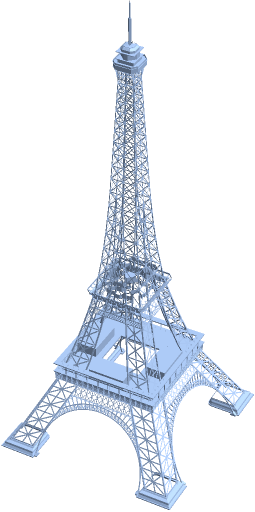
Many systems consist of point interactions. The iconic Eiffel Tower can be modeled through the trusses linking two points with coordinates ${𝒙}_i,{𝒙}_j\in {ℝ}^3$. The unit vector along direction from point $i$ to point $j$ is

Suppose that structure deformation changes the coordinates to ${𝒙}_i+{𝒖}_i$, ${𝒙}_j+{𝒖}_j$. The most important structural response is that on point $i$ a force ${𝒇}_{ij}$ is exerted that can be approximated as

in appropriate physical units. An opposite force ${𝒇}_{ji}=-{𝒇}_{ij}$ acts on point $j$. Note the projector along the truss direction ${𝒍}_{ij}{𝒍}_{ij}^T$. Adding forces on a point from all trusses leads to the linear relation

with $𝒇,𝒖\in {ℝ}^m$, $𝑲\in {ℝ}^{m\times m}$, $d=3$ the number of dimensions, $N$ the number of points, and $m=dN$, the number of degrees of freedom of the structure. Point interactions arise in molecular or social interactions, cellular motility, and economic exchange much in the same form (1). The techniques in this homework are equally applicable to physical chemistry, sociology, biology or business management.

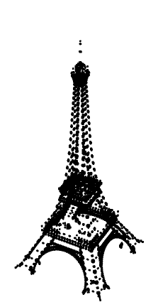
Load the Eiffel Tower data.

octave] 

cd /home/student/courses/MATH547ML/data/EiffelTower;
load EiffelPoints; X=Expression1; [NX,ndims]=size(X);
load EiffelLines; L=Expression1; [NL,nseg]=size(L);

octave] 

m=3*NX; disp([NX NX^2 NL m])

octave] 

Of the possible $N^2\cong 7\times {10}^8$ linkages between points in the structure, only $N_l=31462$ are present. It is wasteful, and often impossible, to store the entire matrix of couplings between points $𝑲\in {ℝ}^{m\times m}$ ($m^2\cong 6\times {10}^9$), but storing only the nonzero elements corresponding to the interacting can be carried out through a sparse matrix. After allocating space with spalloc, the matrix is initialized with zeros along the truss directions.

octave] 

K=spalloc(m,m,3*NL);
for k=1:NL
  i = L(k,1); j = L(k,2);
  p = 3*(i-1)+1; q = 3*(j-1)+1;
  for id=1:3
    for jd=1:3
      K(i+id,j+jd) = 0;
    end;
  end;
end

octave] 

The matrix $𝑲$ can be formed by loops over the trusses. The following computation takes a few minutes. The matrix $K$ has been pre-computed, and can be loaded from a disk file when answering the questions below, rather than executing the following loops.

octave] 

for k=1:NL
  i = L(k,1); j = L(k,2);
  lij = (X(j,:)-X(i,:))'; Pij = lij*lij';
  p = 3*(i-1)+1; q = 3*(j-1)+1;
  for id=1:3
    for jd=1:3
      K(i+id,j+jd) = K(i+id,j+jd) + Pij(id,jd);
    end;
  end;
end

octave] 

save "K.mat" K

octave] 

1.2.Theoretical questions

Provide a proof or counter-example for these true or false questions.

1. If $𝑹$ is an upper-triangular matrix, its singular values are the same as the diagonal values $r_{ii}$.

   Solution. Counterexample

   octave]

   R=[1 1;0 1]

   R =

   1 1

   0 1

   octave]

   svd(R)

   ans =

   1.61803

   0.61803

   octave]

2. If $𝑨={𝑨}^T$, the singular values of $𝑨$ are the same as its eigenvalues.

   Solution. Not quite, singular values are positive, while eigenvalues can be negative. Counterexample

   octave]

   A=[1 0;0 -1]

   A =

   1 0

   0 -1

   octave]

   [svd(A) eig(A)]

   ans =

   1 -1

   1 1

   octave]

3. If $𝑻$ is of full rank, $𝑨$ and $𝑩={𝑻}^{-1}𝑨𝑻$ have the same singular values.

   Solution. No, counterexample

   octave]

   A=[1 2;0 1]; T=[0 2; 1 0]; T1=inv(T); B=T1*A*T; disp([A B])

   1 2 1 0

   0 1 1 1

   octave]

   [svd(A) svd(B)]

   ans =

   2.41421 1.61803

   0.41421 0.61803

   octave]

4. For $𝑨,𝑩\in {ℝ}^{m\times m}$, the matrices $𝑨𝑩$ and $𝑩𝑨$ have the same eigenvalues.

   Solution. Yes. Consider $𝑨𝑩𝒙=\lambda 𝒙$, with $𝒙\ne 𝟎$. Compute

   ${\displaystyle \lambda 𝑩𝒙=𝑩(\lambda 𝒙)=𝑩(𝑨𝑩𝒙)=(𝑩𝑨)(𝑩𝒙).}$

   Set $𝒚=𝑩𝒙$, and obtain

   ${\displaystyle (𝑩𝑨)𝒚=\lambda 𝒚,}$

   the same eigenvalue as for $𝑨𝑩$.

1.3.Reduced order modeling

Load data, and define functions to draw the deformed structure.

octave] 

cd /home/student/courses/MATH547ML/data/EiffelTower;
load EiffelPoints; X=Expression1; [NX,ndims]=size(X);
load EiffelLines; L=Expression1; [NL,nseg]=size(L);
m=3*NX; load K;

octave] 

function drawXu(X,u,L,is)
  clf; view(-30,45); [NX,nd]=size(X);
  [nL,nseg]=size(L); x=[]; y=[]; z=[];
  U=reshape(u,3,NX)';
  for k=1:is:nL
    x=[x X(L(k,1),1)+U(L(k,1),1) X(L(k,2),1)+U(L(k,2),1)];
    y=[y X(L(k,1),2)+U(L(k,1),2) X(L(k,2),2)+U(L(k,2),2)];
    z=[z X(L(k,1),3)+U(L(k,1),3) X(L(k,2),3)+U(L(k,2),3)];
  end;
  plot3(x,y,z);
end

octave] 

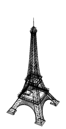
drawXu(X,zeros(m,1),L,20)

octave] 

function drawXU(X,U,L,is)
  clf; view(-30,45); [NX,nd]=size(X);
  [nL,nseg]=size(L); x=[]; y=[]; z=[];
  for k=1:is:nL
    x=[x X(L(k,1),1)+U(L(k,1),1) X(L(k,2),1)+U(L(k,2),1)];
    y=[y X(L(k,1),2)+U(L(k,1),2) X(L(k,2),2)+U(L(k,2),2)];
    z=[z X(L(k,1),3)+U(L(k,1),3) X(L(k,2),3)+U(L(k,2),3)];
  end;
  plot3(x,y,z);
end

octave] 

drawXU(X,zeros(NX,3),L,20)

octave] 

The following questions only require a few Octave lines to solve correctly. Be careful to not request output of the large vectors and matrices that arise. Use visualization with the draw function to represent results, and concentrate on the mathematical formulation. For example, imposing displacement $𝒖=(z,0,0)$ at each node, i.e., a horizontal displacement along the $x$ direction proportional to the $z$ coordinate is accomplished by:

octave] 

U=zeros(NX,3); U(1:NX,1)=X(1:NX,3);

octave] 

drawXU(X,U,L,20)

octave] 

1.3.1.Least squares solution on singular modes

Find the linear combination $𝒔$ of the first 10 singular modes that best approximates a force $𝒇=(z\cos \theta ,z\sin \theta ,0)$ on the structure. Randomly choose $\theta$. Show the first 3 singular modes and the linear combination you find.

Solution. Construct the force at each node, first as an $N\times d$ table, and then as a vector with $m=dN$ components. Check correct representation of the three components of the force as successive elements in a vector.

octave] 

theta=rand()*2*pi; F=zeros(NX,3); 
F(1:NX,1)=X(1:NX,3)*cos(theta); F(1:NX,2)=X(1:NX,3)*sin(theta);
f=reshape(F',m,1); nN=2000; i0=3*(nN-1); disp([F(nN,:)])

octave] 

From the singular value decomposition $𝑲=𝒀𝚺{𝒁}^T\in {ℝ}^{m\times m}$, denote by ${𝒀}_k,{𝒁}_k\in {ℝ}^{m\times k}$ the matrices formed by the first $k$ columns of $𝒀,𝒁$. The matrix $𝒀$ is a basis for the codomain, and the matrix $𝒁$ is a basis for the domain of the linear mapping represented by the matrix $𝑲$. The matrices ${𝒀}_k,{𝒁}_k$ are therefore bases for subspaces within the codomain, domain, respectively. From the full model $𝒇=𝑲𝒖$, obtain a reduced model

with the reduced system matrix defined by

(Note: choosing the same reduced basis for approximation, e.g., $𝒈={𝒁}_k𝒚$, of both forces and displacements is acceptable but not optimal)

Solution of the reduced model gives an approximation of the solution to the full model

If given a force on the full model, the approximation of the force on the reduced model is obtained as the solution of the least squares problem

Since ${𝒀}_k$ has normalized, orthogonal columns, the solution to the least squares problem is $𝒚={𝒀}_k^T𝒇$. Carry out the above steps, through the following five Octave instructions.

octave] 

[Yk,Sigmak,Zk]=svds(K,10);

octave] 

y=Yk'*f; R=Yk'*K*Zk; x=R\y; s=Zk*x;

octave] 

Display the requested singular vectors and the approximate solution obtained from the reduced model. The displacements can be scaled to obtain a more comprehensible visualization.

octave] 

cd /home/student/courses/MATH547ML/homework; mkdir hw04; cd hw04

octave] 

figure(1); drawXu(X,0*Zk(:,1),L,20); print -depsc Fig1a.eps; figure(2);

octave] 

drawXu(X,250*Zk(:,1),L,20); print -depsc Fig1b.eps

octave] 

drawXu(X,250*Zk(:,2),L,20); print -depsc Fig1c.eps

octave] 

drawXu(X,250*Zk(:,3),L,20); print -depsc Fig1d.eps

octave] 

drawXu(X,5000*s,L,20); print -depsc Fig1e.eps

octave] 

Figure 2. Representation of deformation of the Eiffel Tower. Top row contains first 3 singular vectors, showing “squeezing” of the structure along different spatial directions, and the approximation given by the reduced model solution for a force $𝒇=(z\cos \theta ,z\sin \theta ,0)$.

1.3.2.Least squares solution on eigenmodes

Find the linear combination $𝒕$ of the first 10 eigenmodes that best approximates a force $𝒇=(z\cos \theta ,z\sin \theta ,0)$ on the structure. Show the first 3 eigenmodes and the linear combination you find.

Solution. The procedure is similar to the previous case, but with a different choice of bases. The eigenvectors are no longer guaranteed to be be orthogonal, so a $QR$ procedure is applied to obtain the reduced model bases. In this case the basis for the domain and codomain are the same.

octave] 

[Vk,Lambdak]=eigs(K,10); [Rk,Tk]=qr(Vk,0);

octave] 

y=Rk'*f; R=Rk'*K*Rk; x=R\y; t=Rk*x;

octave] 

Display the requested eigenvectors and the approximate solution obtained from the reduced model. Again, the displacements are scaled to obtain a more comprehensible visualization.

octave] 

cd /home/student/courses/MATH547ML/homework; mkdir hw04; cd hw04

octave] 

figure(1); drawXu(X,0*Rk(:,1),L,20); print -depsc Fig2a.eps; figure(2);

octave] 

drawXu(X,250*Rk(:,1),L,20); print -depsc Fig2b.eps

octave] 

drawXu(X,250*Rk(:,2),L,20); print -depsc Fig2c.eps

octave] 

drawXu(X,250*Rk(:,3),L,20); print -depsc Fig2d.eps

octave] 

drawXu(X,5000*t,L,20); print -depsc Fig2e.eps

octave] 

Figure 3. Representation of deformation of the Eiffel Tower. Top row contains first 3 eigenvectors, again showing “squeezing” of the structure along different spatial directions, and the approximation given by the reduced model solution for a force $𝒇=(z\cos \theta ,z\sin \theta ,0)$. Note that the eigenmode reduced solution is very different from that obtained from the singular vector model reduction.

1.3.3.Least squares solution on Krylov modes

Replace singular modes or eigenmodes by orthogonal $𝑸$, with $𝑸𝑹=\left[\begin{array}{ccccc}𝒇& 𝑲𝒇& {𝑲}^2𝒇& \dots & {𝑲}^9𝒇\end{array}\right]$ (known as Krylov modes). Find the linear combination $𝒘$ of the first 10 Krylov modes that best approximates a force $𝒇=(z\cos \theta ,z\sin \theta ,0)$ on the structure. Show the first 3 Krylov modes and the linear combination you find.

Solution. Again, the procedure is similar, but with a different choice of bases. The Krylov modes must be computed and then orthogonalized. In this case also the basis for the domain and codomain are the same.

octave] 

k=10; Kk = [f];
for i=2:k
  Kk = [Kk K*Kk(:,i-1)];
end;
[Wk,Tk]=qr(Kk,0);

octave] 

y=Wk'*f; R=Wk'*K*Wk; x=R\y; w=Wk*x;

octave] 

Display the requested eigenvectors and the approximate solution obtained from the reduced model. Again, the displacements are scaled to obtain a more comprehensible visualization.

octave] 

cd /home/student/courses/MATH547ML/homework; mkdir hw04; cd hw04

octave] 

figure(1); drawXu(X,0*Wk(:,1),L,20); print -depsc Fig3a.eps; figure(2);

octave] 

drawXu(X,250*Wk(:,1),L,20); print -depsc Fig3b.eps

octave] 

drawXu(X,250*Wk(:,2),L,20); print -depsc Fig3c.eps

octave] 

drawXu(X,250*Wk(:,3),L,20); print -depsc Fig3d.eps

octave] 

drawXu(X,250*w,L,20); print -depsc Fig3e.eps

octave] 

Figure 4. Representation of deformation of the Eiffel Tower. Top row contains first 3 Krylov modes, and the approximation given by the reduced model solution for a force $𝒇=(z\cos \theta ,z\sin \theta ,0)$. Note that the Krylov reduced solution does not seem realistic.

Figure 5. Comparison of the first 3 singular modes (top row), eigenmodes (middle row), Krylov modes (bottom row).

1.3.4.Reduced-rank singular mode approximation

From the SVD $𝑲=𝒀𝚺{𝒁}^T$ construct an approximate matrix

and compare the force $𝒇$ with $\stackrel{\sim }{𝒇}=\stackrel{\sim }{𝑲}𝒔$, $𝒔$ from question 1.3.1.

Solution. The previous problem showed the approximate displacement obtained from the reduced model. Here the error in force is estimated

with $c_k={\sigma }_k{𝒛}_k^T𝒔$.

octave] 

c=diag(Sigmak).*Zk'*s;

octave] 

ftilde=Yk*c;

octave] 

norm(f-ftilde)/norm(f)

octave] 

1.3.5.Reduced-rank eigenmode approximation

From the eigendecomposition $𝑲𝑹=𝑹𝚲$ construct an approximate matrix

and compare the force $𝒇$ with $\stackrel{\sim }{𝒇}=\stackrel{\sim }{𝑲}𝒕$, $𝒕$ from question 1.3.2.

Solution. Repeat the above procedure, now using eigenmodes,

with $c_k={\sigma }_k{𝒛}_k^T𝒔$.

octave] 

d=diag(Lambdak).*Rk'*t;

octave] 

ftilde=Rk*d;

octave] 

norm(f-ftilde)/norm(f)

octave] 

1.3.6.Reduced model convergence

Choose one of the reduced models from 1.3.1 to 1.3.4. Repeat the calculations for 15,20,25 modes, and comment on whether the solutions converge.

Solution. Construct a function to return the error in the force estimation for $k$ modes.

octave] 

function ferr=SVDreduced(K,f,k)
  [Yk,Sigmak,Zk]=svds(K,k);
  y=Yk'*f; R=Yk'*K*Zk; x=R\y; s=Zk*x;
  c=diag(Sigmak).*Zk'*s;
  ftilde=Yk*c;
  ferr=norm(f-ftilde)/norm(f);
end

octave] 

ferr10=SVDreduced(K,f,10);

octave] 

ferr15=SVDreduced(K,f,15);

octave] 

ferr20=SVDreduced(K,f,20);

octave] 

ferr25=SVDreduced(K,f,25);

octave] 

disp([ferr10 ferr15 ferr20 ferr25])

octave] 

Notice that the relative error

is decreasing, albeit slowly. Computation of a larger number of singular values (takes a few minutes to complete) leads to a plot from that indicates

octave] 

sig=svds(K,100);

octave] 

plot(log10(sig),'o'); print -depsc Fig6a.eps

octave] 

SVDreduced(K,f,40)

octave]