MATH566 Lesson 6: Polynomial interpolation

Overview

• Polynomial interpolant forms

  • Monomial basis

  • Newton basis

• Interpolation accuracy

• Inexact data

Alternative linear combination bases

• Recall: $f:ℝ\to ℝ$, “difficult” to compute, and known through a sample

  ${\displaystyle 𝒟=\{(x_i,y_i),i=0,1,2,\dots ,m\},y_i=f\left(x_i\right),i\ne j\Rightarrow x_i\ne x_j.}$

• Approximation built from linear combination of $\{g_0\left(t\right),g_1\left(t\right),\dots ,g_n\left(t\right)\}$

  ${\displaystyle g\left(t\right)=c_0{g}_0\left(t\right)+c_1{g}_1\left(t\right)+\cdots +c_n{g}_n{\left(t\right)}_{}}$

• Lagrange basis: $l_i\left(t\right)={\prod }_{j=0}^m{}^{\text{'}}(t-x_j)$ or ${\ell }_i\left(t\right)=\frac{{\prod }_{j=0}^m{}^{\text{'}}(t-x_j)}{{\prod }_{j=0}^m{}^{\text{'}}(x_i-x_j)}$$$

• Monomial basis $\{1,t,t^2,\dots \}$

  ${\displaystyle p\left(t\right)=c_0\cdot 1+c_{1}t+\cdots +c_n{t}^n}$

• Newton basis $\{n_0\left(t\right),\dots ,n_n\left(t\right)\}=\{1,t-x_0,(t-x_0)(t-x_1),\dots \}$

  ${\displaystyle p\left(t\right)=c_0\cdot 1+c_1(t-x_0)+\cdots +c_n(t-x_0)(t-x_1)\dots (t-x_{n-1})}$

Monomial basis compared to Lagrange

• Monomial basis functions are almost indistinguishable over portions of the function domain, closer to linearly dependent than the Lagrange basis functions

• Intuitive analogy from linear algebra: $𝒃\in {ℝ}^m$ can be expressed either in an orthogonal basis $\{{𝒆}_1,\dots ,{𝒆}_m\}$ or a non-orthogonal basis $\{{𝒂}_1,\dots ,{𝒂}_m\}$

  ${\displaystyle 𝒃=b_1{𝒆}_1+\cdots +b_m{𝒆}_m=x_1{𝒂}_1+\cdots +x_m{𝒂}_m\iff 𝒃=𝑨𝒙}$

  When $𝑨$ is close to singular, small errors in $𝒃$ lead to large errors in $𝒙$. Orthogonal bases are preferable.

Newton basis compared to Lagrange

• Behavior similar to monomial basis: almost indistinguishable over portions of the domain.

• Ideally the basis functions $\{g_0\left(t\right),\dots ,g_n\left(t\right)\}$ would be orthonormal with respect to a scalar product with weight $w\left(t\right)$

  ${\displaystyle (g_i,g_j)=\underset{a}{\overset{b}{\int }}w\left(t\right)g_i\left(t\right)g_j\left(t\right)dt={\delta }_{ij}=\{\begin{array}{ll}1& \mathrm{if}i=j\\ 0& \mathrm{if}i\ne j\end{array}.}$

  Compare with vector scalar product ${𝒖}^T𝒗=u_1{v}_1+\cdots +u_m{v}_m{.}_{}$

Coefficients of monomial basis interpolant

• Interpolation conditions $p\left(x_i\right)=c_0+c_1{x}_i+\cdots +c_n{x}_i^n=f\left(x_i\right)=y_i$ lead to

  ${\displaystyle p\left(t\right)=\left[\begin{array}{llll}1& t& \dots & t^n\end{array}\right]\left[\begin{array}{l}{c}_0\\ c_1\\ ⋮\\ c_n\end{array}\right],\left[\begin{array}{llll}1& x_0& \dots & x_0^n\\ 1& x_1& \dots & x_1^n\\ ⋮& ⋮& \ddots & ⋮\\ 1& x_n& \dots & x_n^n\end{array}\right]\left[\begin{array}{l}{c}_0\\ c_1\\ ⋮\\ c_n\end{array}\right]=\left[\begin{array}{l}{y}_0\\ y_1\\ ⋮\\ y_n\end{array}\right]\iff 𝑿𝒄=𝒚.}$

• The matrix $𝑿$ is known as a Vandermonde matrix and though non-singular for distinct sample nodes $(i\ne j\Rightarrow x_i\ne x_j)$, can be become close to singular.

• For given distinct data, the interpolating polynomial is unique

• Coefficients of the monomial basis require solving the linear system, $𝑿𝒄=𝒚$, at $𝒪(n^3/3)$ FLOPs, more expensive than the $𝒪\left(n^2\right)$ for Lagrange form

• Notes:

  • Though $p\left(t\right)=c_0\cdot 1+c_{1}t+\cdots +c_n{t}^n$ is the most often encountered form of a polynomial in analytical mathematics, other forms are more useful in numerical approximation

  • Monomial, Lagrange are different forms of the unique interpolating polynomial

Coefficients of the Newton interpolating polynomial

• Interpolation conditions lead to a triangular system

  ${\displaystyle p\left(t\right)=\left[\begin{array}{llll}{n}_0\left(t\right)& n_1\left(t\right)& \dots & n_n\left(t\right)\end{array}\right]\left[\begin{array}{l}{d}_0\\ d_1\\ ⋮\\ d_n\end{array}\right]\Rightarrow }$ ${\displaystyle \left[\begin{array}{cccc}1& 0& \cdots & 0\\ 1& x_1-x_0& \cdots & 0\\ 1& x_2-x_0& \cdots & 0\\ 1& x_3-x_0& \cdots & 0\\ ⋮& ⋮& \ddots & ⋮\\ 1& x_n-x_0& \cdots & \prod _{j=0}^{n-1}(x_n-x_j)\end{array}\right]\left[\begin{array}{l}{d}_0\\ d_1\\ d_2\\ ⋮\\ d_n\end{array}\right]=\left[\begin{array}{l}{y}_0\\ y_1\\ y_2\\ ⋮\\ y_n\end{array}\right]}$

• Solving the above system now requires $𝒪(n^2/2)$

• The Newton interpolating polynomial arises in finite difference calculus.

Divided differences

• The first few coefficients are

  ${\displaystyle d_0=y_0,d_1=\frac{y_1-d_0}{x_1-x_0}=\frac{y_1-y_0}{x_1-x_0},}$ ${\displaystyle d_2=\frac{y_2-(x_2-x_0)d_1-d_0}{(x_2-x_0)(x_2-x_1)}=\frac{-}{x_2-x_0}.}$

• Introduce divided differences: $\left[y_i\right]=y_i,$

  ${\displaystyle [y_{i+1},y_i]=\frac{\left[y_{i+1}\right]-\left[y_i\right]}{x_{i+1}-x_i}=\frac{y_{i+1}-y_i}{x_{i+1}-x_i},[y_{i+2},y_{i+1},y_i]=\frac{[y_{i+2},y_{i+1}]-[y_{i+1},y_i]}{x_{i+2}-x_i}}$ ${\displaystyle [y_{i+k},y_{i+k-1},\dots ,y_i]=\frac{[y_{i+k},y_{i+k-1},\dots ,y_{i+1}]-[y_{i+k-1},y_{i+k-1},\dots ,y_i]}{x_{i+k}-x_i}}$

• Obtain

  ${\displaystyle p\left(t\right)=\left[y_0\right]\cdot 1+[y_1,y_0]\cdot (t-x_0)+\cdots +[y_n,\dots ,y_0]\cdot (t-x_0)\cdot \dots \cdot (t-x_{n-1}).}$

Interpolation accuracy - an example of numerical analysis

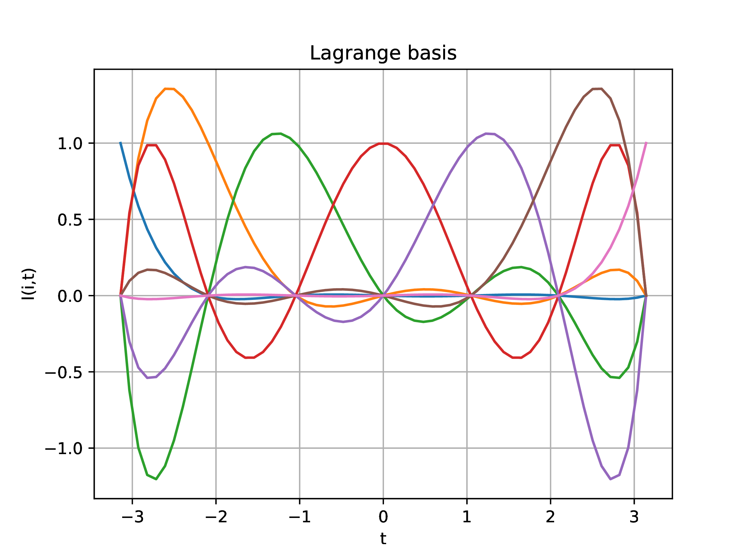
• Polynomial interpolant has no error at sampling nodes, $p\left(x_i\right)=f\left(x_i\right)$

• What about other points. Introduce error function $e\left(t\right)=f\left(t\right)-p\left(t\right)$

• Assume $f\in C^{\infty }\left(ℝ\right)$ (smooth). The error is the reminiscent of Taylor series remainder

  ${\displaystyle f\left(t\right)-p\left(t\right)=\frac{f^{(n+1)}\left({\xi }_t\right)}{(n+1)!}\prod _{i=0}^n(t-x_i)=\frac{f^{(n+1)}\left({\xi }_t\right)}{(n+1)!}w\left(t\right).}$

• Above obtained by repeated application of Rolle's theorem to the function

  ${\displaystyle \Phi \left(u\right)=f\left(u\right)-p\left(u\right)-\frac{f\left(t\right)-p\left(t\right)}{w\left(t\right)}w\left(u\right),}$

• $\Phi \left(u\right)$ $n+2$ has roots at $t,x_0,x_1,\dots ,x_n$, hence its $(n+1)$-order derivative must have a root in the interval $(x_0,x_n)$, denoted by ${\xi }_t$

  ${\displaystyle {\Phi }^{(n+1)}\left({\xi }_t\right)=\frac{d^{n+1}\Phi }{d{u}^{n+1}}\left({\xi }_t\right)=0=f^{(n+1)}\left({\xi }_t\right)-\frac{f\left(t\right)-p\left(t\right)}{w\left(t\right)}(n+1)!}$

• Idea: choose $x_i$ to minimize error. This leads to Chebyshev basis, Lessons 9,10.

Inexact data - Lebesgue constant

• If $y_i=f\left(x_i\right)$ are not known exactly, replace interpolation $p\left(x_i\right)=y_i$ by

  ${\displaystyle g\left(x_i\right)\cong y_i,g\left(x_i\right)=\widehat{y_i}\cong y_i}$

• Define Lebesgue function to expresses deviation from known data,

  ${\displaystyle \lambda \left(t\right)=\sum _{i=0}^n\left|{\ell }_i\left(t\right)\right|}$

• Define the worst case by the Lebesgue constant

  ${\displaystyle \Lambda ={max}_{a⩽t⩽b}\lambda \left(t\right)}$

• The distance between:

  1. the interpolant $p\left(t\right)$, $p\left(x_i\right)=y_i$, and

  2. another approximating polynomial $g\left(t\right)$, $g\left(x_i\right)=$$\widehat{y_i}$, $$

  is bounded by the errors in the data $|y_i-\widehat{y_i}|⩽\delta$ and the Lebesgue constant

  ${\displaystyle {||p-g||}_{\infty }={max}_{a⩽t⩽b}|p\left(t\right)-g\left(t\right)|⩽\Lambda \delta .}$

• The Lebesgue constant depends on the chosen sample nodes.