MATH566 Lesson 8: Piecewise Lagrange polynomial interpolation

Overview

Note: Presentation is simpler than that in textbook

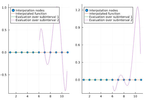
• Interval subpartitions

• Piecewise Lagrange basis

• Analysis: rate of convergence

Interval subpartioning

• Two levels of partitioning for $f:[a,b]\to ℝ$. The idea is to use low-degree polynomials over subintervals.

  • Overall partition $[a,b]={\bigcup }_{j=1}^n[a_j,b_j]$, $a=a_1<a_2<\cdots <a_n=b-l$. Options:

    • If function does not exhibit regions of large variability: uniform partition

      ${\displaystyle a_j=a+(j-1)l,b_j=a_j+l,l=(b-a)/n}$

    • If function varies rapidly in subregions: adaptive partition

  • Interval subpartition, almost always uniform, $m$ chosen small, ($m⩽5$)

    ${\displaystyle [a_j,b_j]=\bigcup _{j=0}^m[a_{ij},b_{ij}],a_{ij}=a_j+ih=b_{i-1,j}}$

    Function sample points are chosen as:

    • For piecewise constant: $x_{0j}=(a_j+b_j)/2$ (midpoint)

    • For $m>0$, $x_{ij}=a_j+i{h}_j$, $h_j=(b_j-a_j)/m$

Piecewise barycentric Lagrange interpolation

• Idea: $m$ sample points over each of $n$ partition intervals:

  • Interpolation can be discontinous at subinterval edges $a_2,\dots ,a_n$

  • Discontinuity in function or derivatives is often required (corners, jumps)

• Over interval $[a_j,b_j]$, barycentric Lagrange interpolation is

  ${\displaystyle p_j\left(t\right)=\frac{\sum _{i=0}^m{y}_{ij}}{\sum _{i=0}^m},w_{ij}=\prod _{k=0,k\ne i}^m\frac{1}{x_{ij}-x_{kj}}}$

• Weights are easily precomputed for uniform subpartitions $x_{ij}=a_j+i{h}_j$

  ${\displaystyle \frac{1}{w_{ij}}=\prod _{k=0,k\ne i}^m{x}_{ij}-x_{kj}={\left(h_j\right)}^m\prod _{k=0}^{i-1}(i-k)\prod _{k=i+1}^m(i-k)\Rightarrow }$ ${\displaystyle \frac{1}{w_{ij}}={(-1)}^{m-i}{\left(h_j\right)}^m\left(\prod _{s=0}^{i}s\right)\left(\prod _{s=1}^{m-i}s\right)={(-1)}^{m-i}{\left(h_j\right)}^{m}i!(m-i)!}$

Piecewise barycentric Lagrange basis

• On interval $[a_j,b_j]$ Lagrange basis is: $\{l_{0j}\left(t\right),\dots ,l_{mj}\left(t\right)\}$, $j=1,\dots ,n$.

• Outside interval $[a_j,b_j]$ set $l_{ij}\left(t\right)=0$, $i=0,1,\dots ,m$.

• Gather into single basis set

  ${\displaystyle \left[\begin{array}{llll}{l}_{01}\left(t\right)& l_{11}\left(t\right)& \dots & l_{m1}\left(t\right)\end{array}\begin{array}{llll}{l}_{02}\left(t\right)& l_{12}\left(t\right)& \dots & l_{m2}\left(t\right)\end{array}\begin{array}{llll}{l}_{0n}\left(t\right)& l_{1n}\left(t\right)& \dots & l_{mn}\left(t\right)\end{array}\right]}$

Figure 1. Two members of a piecewise Lagrange basis of degree 5 over two subintervals