MATH566 Lesson 10: Chebyshev grid interpolation

Overview

Motivation: minimize interpolation error

Here, the best possible behavior of $w\left(t\right)$ is identified.

• Trigonometric expression of Chebyshev weight scalar product

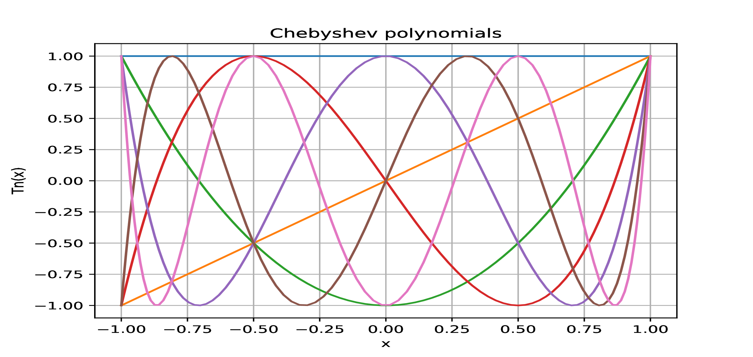
• Chebyshev recurrence relation

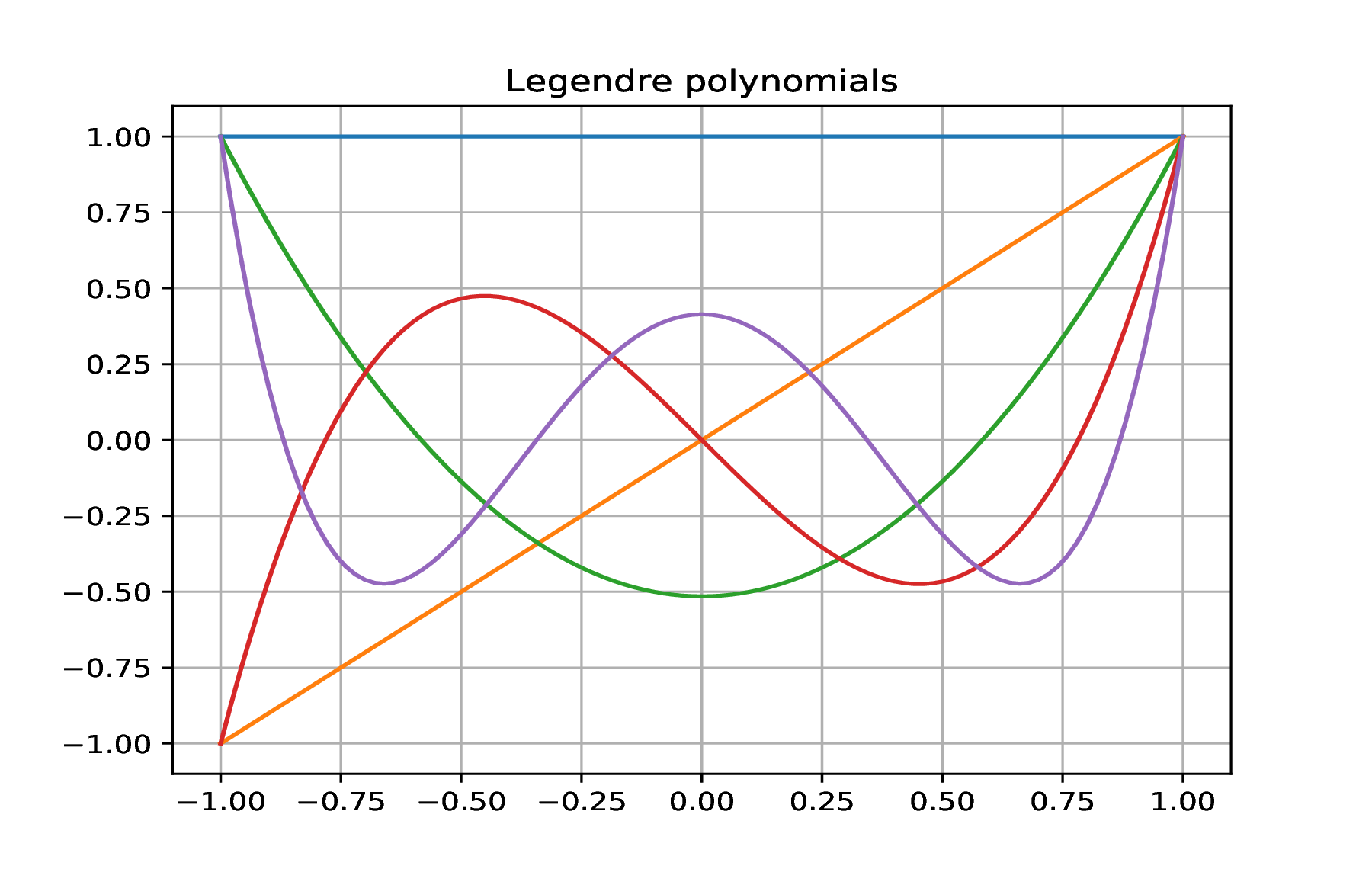
• Roots and extrema of Chebyshev polynomials

• Minimal inf-norm property of Chebyshev polynomials

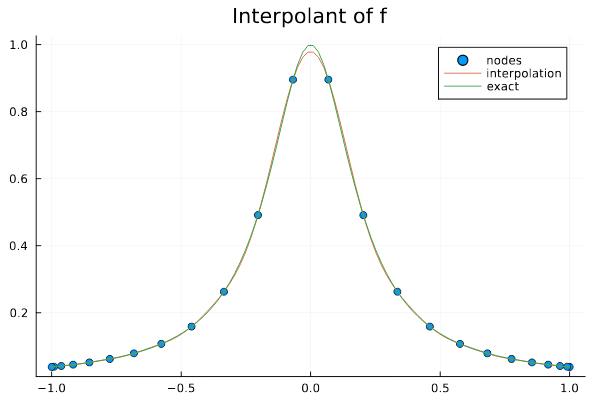
• Runge function on Chebyshev grid

Trigonometric expression of Chebyshev weight scalar product

• Chebyshev polynomials: obtained by orthonormalization of $\{1,t,t^2,\dots \}$ w.r.t

  ${\displaystyle (f,g)=\underset{-1}{\overset{1}{\int }}\frac{f\left(t\right)g\left(t\right)}{\sqrt{1-t^2}}dt.}$

• The Gram-Schmidt process can be applied, but a quicker route is:

  ${\displaystyle t=\cos \theta \Rightarrow dt=-\sin \theta d\theta =-\left(\sqrt{1-{\cos }^2\theta }\right)d\theta =-\left(\sqrt{1-t^2}\right)d\theta \Rightarrow }$ ${\displaystyle (f,g)=\underset{0}{\overset{\pi }{\int }}f\left(t\left(\theta \right)\right)g\left(t\left(\theta \right)\right)d\theta =\underset{0}{\overset{\pi }{\int }}F\left(\theta \right)G\left(\theta \right)d\theta .}$

• Consider $F\left(\theta \right)=\cos (j\theta )$, $G\left(\theta \right)=\cos (k\theta )$ and compute

  ${\displaystyle \underset{0}{\overset{\pi }{\int }}\cos (j\theta )\cos (k\theta )d\theta =c_j{\delta }_{jk},c_0=\pi ,c_j=\frac{\pi }{2}\mathrm{for}j>0}$ ${\displaystyle }$

Chebyshev recurrence relationship

• Introduce notation $T_n\left(t\left(\theta \right)\right)=\cos (n\theta )$ (un-normalized Chebyshev polynomial)

• Observe: $T_0\left(t\right)=1$, $T_1\left(t\right)=\cos \theta =t$,

  ${\displaystyle T_{n+1}\left(t\left(\theta \right)\right)+T_{n-1}\left(t\left(\theta \right)\right)=\cos \left[(n+1)\theta \right]+\cos \left[(n+1)\theta \right]=2\cos \theta \cos (n\theta )}$

• The above trigonometric identity leads to the recurrence relationship

  ${\displaystyle T_{n+1}\left(t\right)=2t{T}_n\left(t\right)+T_{n-1}}$

• Since $T_0\left(t\right)=1$, $T_1\left(t\right)=t$, recurrence relationship implies $T_n\left(t\right)$ are polynomials

  ${\displaystyle T_2\left(t\right)=2t^2-1,T_3\left(t\right)=4t^3-3t,T_4\left(t\right)=8t^4-8t^2+1,\dots }$

• Unit-norm Chebyshev polynomials are $T_n\left(t\right)/c_n$, $c_0=\pi$, $c_j=\frac{\pi }{2},j>1$

  ${\displaystyle (T_m,T_n)=\underset{-1}{\overset{1}{\int }}\frac{T_m\left(t\right)T_n\left(t\right)}{\sqrt{1-t^2}}dt=\underset{0}{\overset{\pi }{\int }}\cos (m\theta )\cos (n\theta )d\theta =c_n{\delta }_{mn}.}$

Minimal inf-norm property of Chebyshev polynomials

• Chebyshev polynomials and the behavior of $w\left(t\right)={\prod }_{j=0}^n(t-x_j)$

• Introduce inf-norm ${||f||}_{\infty }={max}_{-1⩽t⩽1}\left|f\left(t\right)\right|$

• Monic form of Chebyshev polynomials: $P_0\left(t\right)=1$, $P_n\left(t\right)=2^{1-n}{T}_n\left(t\right)$

  ${\displaystyle T_0\left(t\right)=1,T_1\left(t\right)=t,T_2\left(t\right)=2t^2-1,T_3\left(t\right)=4t^3-3t,T_4\left(t\right)=8t^4-8t^2+1,\dots }$

  Coefficient of term of $n^{\mathrm{th}}$ degree in $P_n\left(t\right)$ is one (monic polynomial) like $w\left(t\right)$

  ${\displaystyle ||P_0\left(t\right)||=1,{||P_n\left(t\right)||}_{\infty }=2^{1-n},n>0}$

• Intuitively: Runge function overshoot of interpolant near interval endpoints

  ${\displaystyle f\left(t\right)=\frac{1}{1+{(5t)}^2},f\left(t\right)-p_n\left(t\right)=\frac{f^{(n+1)}\left({\xi }_t\right)}{(n+1)!}w\left(t\right),w\left(t\right)=\prod _{j=0}^n(t-x_j)}$

  is not due to $f^{(n+1)}\left({\xi }_t\right)$ (very smooth), but to $w\left(t\right)$, i.e., choice of $x_j$

• What monic polynomial has the smallest inf-norm? The Chebyshev polynomial.

Inf-norm of monic polynomials theorem

Theorem. $p:[-1,1]\to ℝ$, monic polynomial of degree $n$ has a inf-norm lower bound

Proof. By contradiction, assume the monic polynomial $p:[-1,1]\to ℝ$ has ${||p||}_{\infty }<2^{1-n}$. Construct a comparison with the Chebyshev polynomials by evaluating $p$ at the extrema $x_j=\cos (j\pi /n)$,

Since the above states ${(-1)}^{j}p\left(x_j\right)<{(-1)}^j{P}_n\left(x_j\right)$ deduce

However, $p,P_n$ both monic implies that $p\left(x_j\right)-P_n\left(x_j\right)$ is a polynomial of degree $n-1$ that would change signs $n$ times to satisfy (1), and thus have $n$ roots contradicting the fundamental theorem of algebra.$\square$

Chebyshev grids minimizes interpolation error, even for Runge function

• For polynomial interpolant of degree $n$ of $f:[-1,1]\to ℝ$ choose error term

  ${\displaystyle w\left(t\right)=\prod _{j=0}^n(t-z_j)=T_{n+1}\left(t\right),z_j=\cos {\theta }_j,{\theta }_j=\frac{\pi (2j+1)}{2(n+1)},j=0,1,\dots ,n.}$ ${\displaystyle 𝒵=\{(z_j,f\left(z_j\right)),j=0,1,\dots ,n\}}$

• Alternatively, roots of $T_n^{\text{'}}\left(t\right)=n{U}_{n-1}\left(t\right)$, $U_{n-1}\left(t\right)=\sin (n\theta )/\sin \theta$ and $\pm 1$

  ${\displaystyle w\left(t\right)=\prod _{j=0}^n(t-x_j),x_j=-\cos {\phi }_j,{\phi }_j=\frac{j\pi }{n},j=0,1,\dots ,n}$ ${\displaystyle 𝒟=\{(x_j,f\left(x_j\right)),j=0,1,\dots ,n\}}$

Figure 2. Chebyshev grid interpolant of degree 23

Barycentric form of Chebyshev interpolant

• Numerical methods suggested an orthogonal basis set $\{T_0,T_1,\dots \}$

• Numerical analysis has furnished an optimal set of sample points $x_j$ or $z_j$

• Still to study: computational complexity

• Naïve approach: $f\left(t\right)\cong p\left(t\right)={\sum }_{j=0}^n{c}_j{T}_j\left(t\right)$, apply interpolation conditions

  ${\displaystyle y_j=f\left(x_j\right)=p\left(x_j\right)\Rightarrow \left[\begin{array}{llll}{T}_0\left(𝒙\right)& T_1\left(𝒙\right)& \dots & T_n\left(𝒙\right)\end{array}\right]𝒄=𝒚\iff 𝑨𝒄=𝒚}$

  obtaining a linear system with a full matrix at computational cost $𝒪(n^3/3)$

• Recall: polynomial interpolant is unique. Use Lagrange barycentric form

  ${\displaystyle p\left(t\right)=\sum _{j=0}^n{y}_j\frac{w_j}{t-x_j}/\sum _{j=0}^n{y}_j\frac{w_j}{t-x_j}.}$

• When sample points are $x_j=-\cos {\phi }_j,{\phi }_j=\frac{j\pi }{n},j=0,1,\dots ,n$, weights are

  ${\displaystyle w_j={(-1)}^j,j=1,\dots ,m-1,w_0=1/2,w_n={(-1)}^n/2}$

  favoring data set $𝒟=\left\{(x_j,f\left(x_j\right))\right\}$ over $𝒵=\left\{(z_j,f\left(z_j\right))\right\}$, $j=0,1,\dots ,n$.