MATH566 Lesson 11: Least squares approximation

Overview

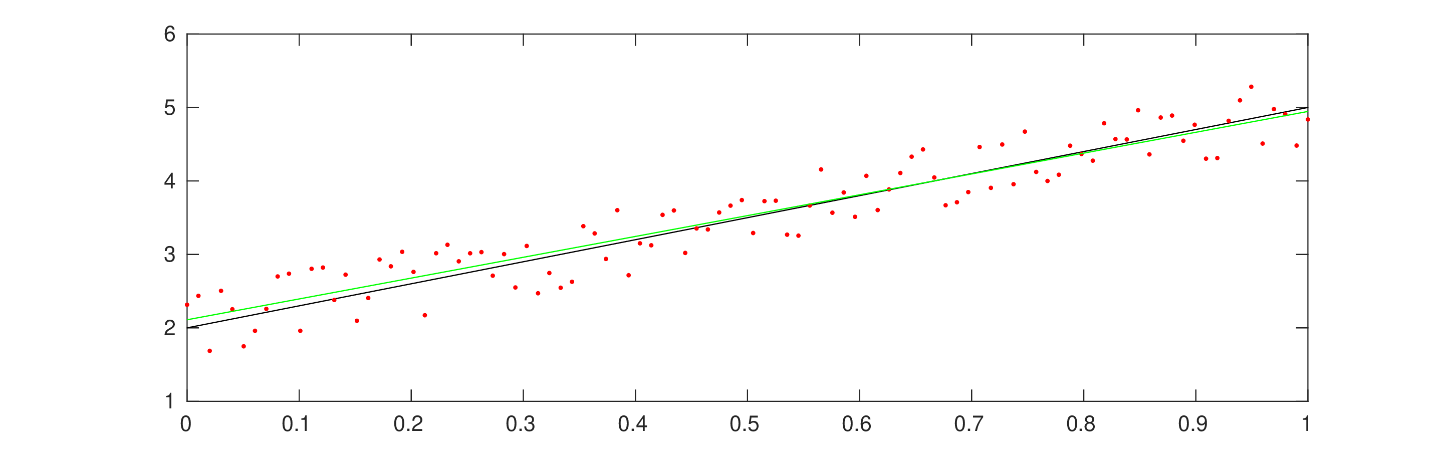
Motivation: data points might be affected by errors. The interpolation criterion $y_i=f\left(x_i\right)=g\left(x_i\right)$, i.e., exactly recover the function values is not appropriate.

• Minimal norm approximation criteria

• Solving linear least squares problems

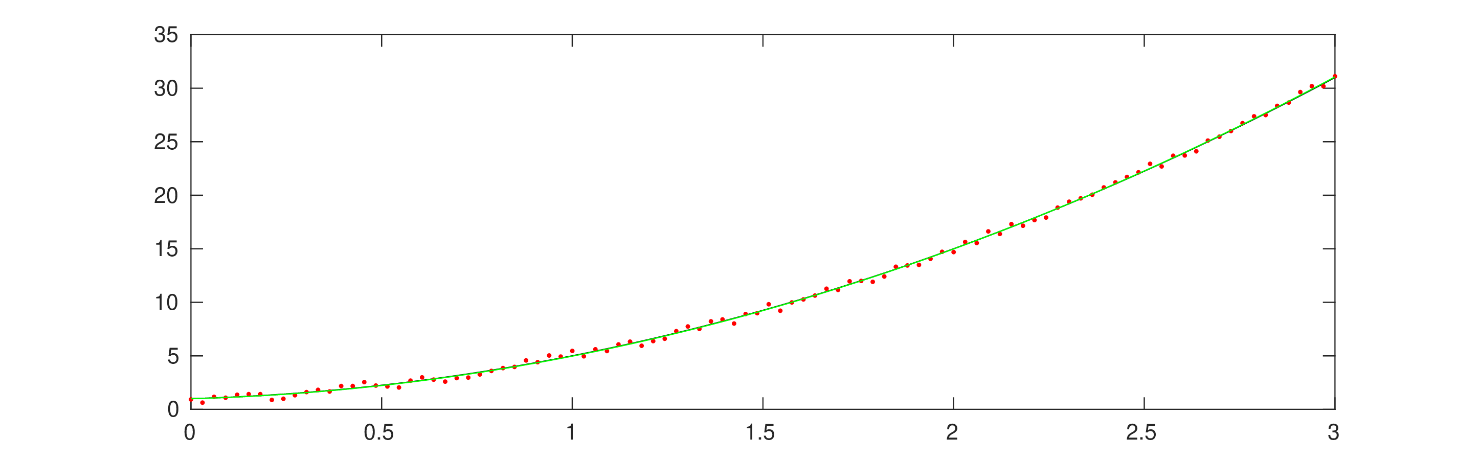
• Nonlinear least squares problems

Minimal norm approximation criteria

• Problem: approximate $f:[a,b]\to ℝ$ by $g:[a,b]\to ℝ$, $f\left(t\right)\cong g(t;c)$, $c$ are approximant parameters

• Best approximants can be defined in terms of error minimization

  ${\displaystyle \epsilon =||f-g||,{min}_c\epsilon \left(c\right)}$

• Examples. Assume $f$ known by sample $𝒟=\{(x_i,y_i=f\left(x_i\right)),i=1,\dots ,m\}$

  • Interpolation: ${||f||}_i={\sum }_{i=1}^m\left|f\left(x_i\right)\right|$. Verify norm properties:

    • $a\in ℝ$, ${||af||}_i=$${\sum }_{i=1}^m|af\left(x_i\right)|=\left|a\right|{\sum }_{i=1}^m\left|f\left(x_i\right)\right|=\left|a\right|{||f||}_i?$

    • ${||f||}_i=0={\sum }_{i=1}^m\left|f\left(x_i\right)\right|\Rightarrow f\left(x_i\right)=0\Rightarrow f=0$ on grid $\{x_1,\dots ,x_m\}$

    • $||f+g||={\sum }_{i=1}^m|f\left(x_i\right)+g\left(x_i\right)|⩽$${\sum }_{i=1}^m(\left|f\left(x_i\right)\right|+\left|g\left(x_i\right)\right|)={||f||}_i+{||g||}_i$

  • Least-sqaures: use 2-norm ${||f||}_2={\sum }_{i=1}^m{\left(f\left(x_i\right)\right)}^2$

  • Min-max: use inf norm ${||f||}_{\infty }={max}_{a⩽t⩽b}\left|f\left(t\right)\right|$

    ${\displaystyle {min}_c\epsilon \left(c\right)\Rightarrow {min}_c{max}_{a⩽t⩽b}|f\left(t\right)-g(t;c)|.}$

Linear least squares

• Based on two ideas:

  1. Approximant is a linear combination, $g=c_1{g}_2+\cdots +c_n{g}_n$

  2. Error is measured by 2-norm

     ${\displaystyle {min}_{𝒄\in {ℝ}^n}||f-g||\Rightarrow {min}_{c\in {ℝ}^n}\sum _{i=1}^m{(y_i-g(x_i;c))}^2.}$

• Choose a basis set:

  • Monomial ${ℳ}_n\left(t\right)=\{1,t,t^2,\dots ,t^{n-1}\}$

  • Trigonometric $𝒯=\{1,\cos t,\sin t,\dots \}$, $f:[0,2\pi ]\to ℝ$, $f(t+2\pi )=f\left(t\right)$

  • Exponential ${ℰ}_n\left(t\right)=\{1,e^t,e^{2t},\dots ,e^{(n-1)t}\}$

• Evaluate basis set at grid points $𝒙\in {ℝ}^m$, obtain $𝑨\in {ℝ}^{m\times n}$ matrix

  ${\displaystyle {ℳ}_n\left(𝒙\right)=𝑨=\left[\begin{array}{lllll}𝟏& 𝒙& {𝒙}^2& \dots & {𝒙}^{n-1}\end{array}\right],{𝒙}^k={\left[\begin{array}{lll}{x}_1^k& \dots & x_m^k\end{array}\right]}^T}$

• Seek $𝒄\in {ℝ}^n$ ${min}_{𝒄\in {ℝ}^n}{||𝒚-𝑨𝒄||}_2$

Orthogonal projection in linear spaces

• Projection of $𝒗\in {ℝ}^m$ along direction $𝒖\in {ℝ}^m$, $||𝒖||=1$

  Figure 1. Projection operation

• $𝒘=(||𝒗||\cos \theta )𝒖=(||𝒗||)𝒖=({𝒖}^T𝒗)𝒖=𝒖\left({𝒖}^T𝒗\right)=(𝒖{𝒖}^T)𝒗\Rightarrow$

• Projection matrix ${𝑷}_{𝒖}=𝒖{𝒖}^T$

Projection examples

• Projection along ${𝒆}_1$ direction in ${ℝ}^2$

  ${\displaystyle {𝑷}_{{𝒆}_1}=\left[\begin{array}{l}1\\ 0\end{array}\right]\left[1\begin{array}{ll}& 0\end{array}\right]=\left[\begin{array}{ll}1& 0\\ 0& 0\end{array}\right],{𝑷}_{{𝒆}_1}\left[\begin{array}{l}{x}_1\\ x_2\end{array}\right]=\left[\begin{array}{ll}1& 0\\ 0& 0\end{array}\right]\left[\begin{array}{l}{x}_1\\ x_2\end{array}\right]=\left[\begin{array}{l}{x}_1\\ 0\end{array}\right].}$

• Projection along direction of vector $𝒘=\left[\begin{array}{l}1\\ 1\\ 1\end{array}\right]$ in ${ℝ}^3$:

  • First obtain a vector of unit norm $𝒖=𝒘/||𝒘||=\frac{1}{\sqrt{3}}$ $\left[\begin{array}{l}1\\ 1\\ 1\end{array}\right]$

  • Projection matrix

    ${\displaystyle {𝑷}_{𝒖}=𝒖{𝒖}^T=\frac{1}{3}\left[\begin{array}{l}1\\ 1\\ 1\end{array}\right]\left[\begin{array}{lll}1& 1& 1\end{array}\right]=\frac{1}{3}\left[\begin{array}{lll}1& 1& 1\\ 1& 1& 1\\ 1& 1& 1\end{array}\right].}$

Geometric solution of least squares problem

• Linear least squares problems (LLSQ) easily solved by Pythagorean theorem

  

• Solution is orthgonal projection onto $C\left(𝑨\right)$

  ${\displaystyle 𝑸𝑹=𝑨,{𝑷}_{C\left(𝑨\right)}=𝑸{𝑸}^T,𝒗=(𝑸{𝑸}^T)𝒚}$

• The LLSQ parameter vector $𝒄$ is found by back-substitution from

  ${\displaystyle 𝒗=(𝑸{𝑸}^T)𝒚=(𝑸𝑹)𝒄\Rightarrow 𝑹𝒄={𝑸}^T𝒚.}$

LLSQ polynomial approximants

• Consider data $𝒟=\{(x_i,y_i),i=1,\dots ,m\}$

• The polynomial interpolant of degree $m-1$ passes through the data points

  ${\displaystyle p_{m-1}\left(x\right)=c_0+c_{1}x+\cdots +c_{m-1}{x}^{m-1}=\left[\begin{array}{llll}1& x& \dots & x^{m-1}\end{array}\right]𝒄}$

• Impose conditions $p_{m-1}\left(x_i\right)=y_i,i=1,\dots ,m$ to obtain linear system

  ${\displaystyle \left[\begin{array}{lllll}1& x_1& x_1^2& \dots & x_1^{m-1}\\ 1& x_2& x_2^2& \dots & x_2^{m-1}\\ ⋮& ⋮& ⋮& \ddots & ⋮\\ 1& x_m& x_m^2& \dots & x_m^{m-1}\end{array}\right]\left[\begin{array}{l}{c}_0\\ c_1\\ c_2\\ ⋮\\ c_{m-1}\end{array}\right]=\left[\begin{array}{l}{y}_1\\ y_2\\ y_3\\ ⋮\\ y_m\end{array}\right]\Rightarrow 𝑨𝒄=𝒚,𝑨\in {ℝ}^{m\times m}}$

  >>	m=4; x=transpose(1:m); y=1 - 2*x + 3*x.^2 - 4*x.^3;

  >>	A=[x.^0 x.^1 x.^2 x.^3]; [Q,R]=qr(A); c = R \ (Q'*y); c'

  ${\displaystyle \left(\begin{array}{cccc}1.0000& -2.0000& 3.0000& -4.0000\end{array}\right)}$

Linear regression

• Consider noisy data containing many measurements $𝒟=\{(x_i,y_i),i=1,\dots ,m\}$

• Assume data without noise would conform to some polynomial law

  ${\displaystyle y_i=z_i+r_i=c_0+c_1{x}_i+r_i,i=1,\dots ,m}$

  with $r_i$ a random number uniformly distributed within $(-R,R)$.

LSQ parabolic approximant

• Consider noisy data containing many measurements $𝒟=\{(x_i,y_i),i=1,\dots ,m\}$

• Assume data without noise would conform to some polynomial law

  ${\displaystyle y_i=z_i+r_i=c_0+c_1{x}_i+r_i,i=1,\dots ,m}$

  with $r_i$ a random number uniformly distributed within $(-R,R)$.

  >>	m=100; x=linspace(0,3,m)';

  >>	c0=1; c1=1; c2=3; z=c0+c1*x+c2*x.^2; y=(z+rand(m,1)-0.5);

  >>	A=ones(m,3); A(:,2)=x(:); A(:,3)=x(:).^2; [Q,R]=qr(A); c=R\(Q'*y); c'

  ${\displaystyle \left(\begin{array}{ccc}1.0047& 0.9641& 3.0143\end{array}\right)}$

  >>	w=A*c; plot(x,z,'k',x,y,'.r',x,w,'g');