MATH590

MATH590: Approximation in $ℝ^{d}$

Abstract

The methods of mathematical analysis are used to process data acquired from cell-phone accelerometers and gyroscopes to: (1) reconstruct the trajectory of the person carrying the cell-phone along a pre-determined path, and (2) determine data features that might identify the person.

1 Kinematics of rigid body motion ?

1.1Reference frames ?

1.2Matrix representation of rotations ?

1.3Matrix representation of infinitesimal rotations in relative coordinate system ?

1.4Change in the orientation of the relative coordinate system ?

1.5Change in position of the relative coordinate system ?

2Qualitative data analysis ?

2.1Data input ?

2.2Data plotting ?

2.2.1Linear accelerations ?

2.2.2Angular accelerations ?

3Trajectory reconstruction ?

3.1Integration ?

3.1.1Reconstructing angular velocities from gyroscope measurements ?

3.1.2Reconstructing the relative coordinate system basis ?

3.1.3Reconstructing the walker velocity and position ?

4Trajectory analysis ?

4.1Interpolation ?

4.2Least squares ?

4.3Min-max ?

1 Kinematics of rigid body motion

Some basic theory on the kinematics of rigid body motion is necessary to process the acceleration data obtained from the Physics Toolbox Android application. It is assumed that the cell phone and walker form a rigid body, i.e., the cell phone is held rigidly at constant orientation. Note that this hypothesis is likely to be affected by natural flexural motions of the wrist and elbow.

1.1Reference frames

Describing the kinematics (i.e., motion without consideration of forces) requires consideration of two reference frames:

Absolute reference frame: A fixed coordinate system, i.e., with origin at the starting point of the walk and fixed axis orientations.
Relative reference frame: A moving coordinate system, carried by and centered on the sensor (i.e., cell-phone) motion, with variable axis orientations.

The notation for kinematic quantitites in the two reference systems is presented in Table 1, with a depiction represented in Figure 1. In particular, $𝚯, 𝛀$ are the orientation, angular velocity of the relative system expressed as rotation angles, angular velocities around the axes of the absolute system $𝐄$ . The orientation expressed as rotation angles in the relative coordinate system $𝐔$ are denoted by $𝜽$ , and $𝝎$ are the corresponding angular velocities.

Reference frame	Absolute	Relative	Relationships
Basis vectors	$𝐄 = (\begin{array}{lll} 𝒆_{1} & 𝒆_{2} & 𝒆_{3} \end{array})$	$𝐔 = (\begin{array}{lll} 𝒖_{1} & 𝒖_{2} & 𝒖_{3} \end{array})$	$𝐔 = 𝐑_{(φ, 𝒍)} 𝐄$
Origin	$𝑶 = (0, 0, 0)$	$𝑿 (t)$
Orientation	$𝚯$	$𝜽$
Linear velocity		$𝑽 = \dot{𝑿}$
Angular velocity	$𝛀 = \dot{𝚯}$	$𝝎 = \dot{𝜽}$
Linear acceleration		$\dot{𝑽} = \ddot{𝑿}$
Angular acceleration	$\dot{𝛀} = \ddot{𝚯}$	$𝜺 = \dot{𝝎}$

Table 1. Kinematic quantitites in the absolute, relative reference frames

Figure 1. Absolute reference system $(O, 𝐄)$ , cell phone position $C$ , relative reference system $(C, 𝐔)$

1.2Matrix representation of rotations

During motion, the orientation of the relative reference frame changes due to rotation of the walker. There exists some axis $𝒍$ and angle of rotation $φ$ around the axis $𝒍$ that transforms the original orientation $𝐄$ into the current orientation of the relative coordinate system $𝐔$ ,

𝐔 = 𝐑_{(φ, 𝒍)} 𝐄 .

(1)

The Euler representation of a rotation matrix is

𝐑_{(φ, 𝒍)} = \cos φ (𝐄 - 𝒍 \otimes 𝒍) - \sin φ (𝝐 𝒍) + 𝒍 \otimes 𝒍,

(2)

where $𝝐$ is the completely anti-symmetric Levi-Civita tensor with components

ϵ_{i j k} = sign (\begin{array}{lll} 1 & 2 & 3 \\ i & j & k \end{array}),

(3)

the sign of the permutation of $(1, 2, 3)$ into $(i, j, k)$ . The contraction of the rank-3 Levi-Civita tensor with a vector results in a rank-2 tensor (i.e., a matrix)

𝝐 𝒍 = (\begin{array}{lll} 0 & l_{3} & - l_{2} \\ - l_{3} & 0 & l_{1} \\ l_{2} & - l_{1} & 0 \end{array}) .

1.3Matrix representation of infinitesimal rotations in relative coordinate system

For an infinitesimal rotation $d φ$ , $\sin (d φ) ≅ d φ$ , $\cos (d φ) ≅ 1$ , and the rotation matrix becomes

𝐑_{(d φ, 𝒍)} = 𝐄 + d 𝐒,

(4)

where $d 𝐒 = - d φ (𝝐 𝒍)$ , and has inverse

𝐑_{(d φ, 𝒍)}^{- 1} = 𝐑_{(d φ, 𝒍)}^{T} = 𝐄 - d 𝐒 .

(5)

Consider now the rotation matrix $𝐐$ that corresponds to the composition of three infinitesimal rotations around axes $(𝒍_{1}, 𝒍_{2}, 𝒍_{3})$

𝐐 = 𝐑_{(d φ_{1}, 𝒍_{1})} 𝐑_{(d φ_{2}, 𝒍_{2})} 𝐑_{(d φ_{3}, 𝒍_{3})} = (𝐄 + d 𝐒_{1}) (𝐄 + d 𝐒_{2}) (𝐄 + d 𝐒_{3}) ≅ 𝐄 + d 𝐒_{1} + d 𝐒_{2} + d 𝐒_{3} .

(6)

For infinitesimal rotations $(d θ_{1}, d θ_{2}, d θ_{3})$ around the axes of the relative coordinate system $(𝒖_{1}, 𝒖_{2}, 𝒖_{3})$ , the composite rotation matrix is

𝐐 = 𝐄 + d 𝐒 = (\begin{array}{lll} 1 & 0 & 0 \\ 0 & 1 & 0 \\ 0 & 0 & 1 \end{array}) + (\begin{array}{lll} 0 & - d θ_{3} & d θ_{2} \\ d θ_{3} & 0 & - d θ_{1} \\ - d θ_{2} & d θ_{1} & 0 \end{array}) .

(7)

1.4Change in the orientation of the relative coordinate system

During the infinitesimal time step $d t$ the relative coordinate axes undergo a rotation

𝐔 (t + d t) = 𝐐 𝐔 (t) = (𝐄 + d 𝐒) 𝐔 (t),

which gives a differential system

\dot{𝐔} = \dot{𝐒} 𝐔,

(8)

describing the change in the relative system orientation in terms of the rotation velocities around the axes of the relative system

\dot{𝐒} (𝝎) = (\begin{array}{lll} 0 & - ω_{3} & ω_{2} \\ ω_{3} & 0 & - ω_{1} \\ - ω_{2} & ω_{1} & 0 \end{array}) .

(9)

The current orientation of the relative coordinate system $𝐔 (t)$ is the solution of the initial value problem (IVP)

\begin{array}{lll} \dot{𝝎} & = & 𝜺, \\ \dot{𝐔} & = & (\begin{array}{lll} 0 & - ω_{3} & ω_{2} \\ ω_{3} & 0 & - ω_{1} \\ - ω_{2} & ω_{1} & 0 \end{array}) 𝐔, \\ 𝐔 (0) & = & 𝐄, \\ 𝝎 (0) & = & 𝟎 . \end{array}

1.5Change in position of the relative coordinate system

The cell-phone measures accelerations $𝒂$ along axes of the relative coordinate system, that are expressed in the global coordinate system as

\ddot{𝑿} = 𝐔 𝒂 .

The overall IVP to find the position is

\begin{array}{lll} \dot{𝝎} & = & 𝜺, \\ \dot{𝐔} & = & (\begin{array}{lll} 0 & - ω_{3} & ω_{2} \\ ω_{3} & 0 & - ω_{1} \\ - ω_{2} & ω_{1} & 0 \end{array}) 𝐔, \\ \dot{𝑿} & = & 𝑽, \\ \dot{𝑽} & = & 𝐔 𝒂, \\ 𝝎 (0) & = & 𝟎, \\ 𝐔 (0) & = & 𝐄, \\ 𝑿 (0) & = & 𝟎, \\ 𝑽 (0) & = & 𝟎, \end{array}

(10)

where the linear, angular accelerations $𝒂, 𝜺$ are known from measurements.

2Qualitative data analysis

A first step in processing the data $(𝒂, 𝜺)$ acquired from the cell phone is to carry out some basic qualitative analysis, shown here using Octave (Matlab clone).

2.1Data input

Cell-phone data saved in CSV format is read in and examined through the following steps:

Set the current directory

octave>

dir='/home/student/courses/MATH590/NUMdata';

chdir(dir);

octave>

Read the CSV-formatted data, and find the size of the data

octave>

data=csvread('Mitran.csv');

[m,d] = size(data); disp([m d]);

18841 8

octave>

Visually examine some of the data

octave>

data(1:10,:)

$(\begin{array}{cccccccc} 0 & 0 & 0 & 0 & 0 & 0 & 0 & 0 \\ 0.004 & - 0.7803 & 0.2999 & - 1.799 & - 0.1402 & 0.2944 & 0.0533 & 0 \\ 0.005 & - 0.7803 & 0.2999 & - 1.799 & 0.0015 & 0.3671 & 0.2121 & 0 \\ 0.005 & - 0.0953 & 0.0762 & - 0.0111 & 0.0015 & 0.3671 & 0.2121 & 0 \\ 0.006 & - 0.0953 & 0.0762 & - 0.0111 & 0.0015 & 0.3671 & 0.2121 & 0 \\ 0.006 & - 0.0953 & 0.0762 & - 0.0111 & 0.0015 & 0.3671 & 0.2121 & 0 \\ 0.006 & - 0.0953 & 0.0762 & - 0.0111 & 0.0015 & 0.3671 & 0.2121 & 0 \\ 0.006 & - 0.0953 & 0.0762 & - 0.0111 & 0.0015 & 0.3671 & 0.2121 & 0 \\ 0.006 & - 0.0953 & 0.0762 & - 0.0111 & 0.0015 & 0.3671 & 0.2121 & 0 \\ 0.007 & - 0.0953 & 0.0762 & - 0.0111 & - 0.0003 & 0.7379 & - 0.0279 & 0 \end{array})$

octave>

Each line contains $(t_{k}, 𝒂_{k}, 𝜺_{k})$ , with $t_{k}$ the elapsed time, $𝒂_{k}$ the linear accelation at time $t_{k}$ , $𝜺_{k}$ the angular acceleration at time $t_{k}$ . Note that there are several repeated $t_{k}$ values. Since solving the IVP (10) requires definition of the functions $(𝒂 (t), 𝜺 (t))$ , some initial processing is required to eliminate duplicate values. The Octave unique function is used to obtain a vector t of the mu unique values, and the indices iu at which each unique value is first encountered.

octave>

[t,iu]=unique(data(:,1));

octave>

t(1:10)'

$(\begin{array}{cccccccccc} 0 & 0.004 & 0.005 & 0.006 & 0.007 & 0.025 & 0.056 & 0.068 & 0.101 & 0.119 \end{array})$

octave>

iu(1:16)'

$(\begin{array}{cccccccccccccccc} 1 & 2 & 4 & 9 & 11 & 12 & 15 & 18 & 19 & 20 & 22 & 24 & 25 & 26 & 28 & 31 \end{array})$

octave>

mu=max(size(iu))

$14190$

octave>

t(mu-6:mu)'

$(\begin{array}{ccccccc} 162.851 & 162.852 & 162.88 & 162.881 & 162.91 & 162.93 & 162.944 \end{array})$

octave>

iu(mu-6:mu)'

$(\begin{array}{ccccccc} 18830 & 18831 & 18832 & 18834 & 18837 & 18838 & 18841 \end{array})$

octave>

raddeg=pi/180

$0.017453$

octave>

Define vectors a, epsilon containing unique linear, angular acceleration values.

octave>

a=data(iu,2:4); epsilon=data(iu,5:7)/raddeg;

octave>

[a(1:6,:) epsilon(1:6,:)]

$(\begin{array}{cccccc} 0 & 0 & 0 & 0 & 0 & 0 \\ - 0.7803 & 0.2999 & - 1.799 & - 8.0329 & 16.868 & 3.0539 \\ - 0.0953 & 0.0762 & - 0.0111 & 0.085944 & 21.033 & 12.152 \\ - 0.0953 & 0.0762 & - 0.0111 & 0.085944 & 21.033 & 12.152 \\ - 0.6242 & - 0.0203 & - 0.9742 & - 0.017189 & 42.279 & - 1.5986 \\ - 0.6242 & - 0.0203 & - 0.9742 & - 0.017189 & 42.279 & - 1.5986 \end{array})$

octave>

data(1:10,:)

octave>

2.2Data plotting

Having ensured data corresponds to functions $𝒂 (t), 𝜺 (t)$ , a next step is data visualization. This shall be accomplished by writing the data to a text file and using the Gnuplot utility.

octave>

fid=fopen('Mitran.data','w');

fprintf(fid,'%f %f %f %f %f %f %f\n',[t a epsilon]');

fclose(fid);

octave>

2.2.1Linear accelerations

GNUplot]

cd '/home/student/courses/MATH590/NUMdata'

set terminal postscript eps enhanced color

set style line 1 lt 2 lc rgb "red" lw 3

set style line 2 lt 2 lc rgb "green" lw 3

set style line 3 lt 2 lc rgb "blue" lw 3

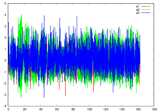
plot 'Mitran.data' u 1:2 w l ls 1 title "a1", ” u 1:3 w l ls 2 title "a2", ” u 1:4 w l ls 3 title "a3"

GNUplot]

Observations on the above plot (qualitative data analysis):

average accelerations seem to be zero as expected for a closed path. This can readily be checked

octave>

mean(a)

$(\begin{array}{ccc} 0.014903 & 0.11257 & 0.065759 \end{array})$

octave>

std(a)

$(\begin{array}{ccc} 0.68179 & 1.2446 & 0.97412 \end{array})$

octave>

mean(a)./std(a)

$(\begin{array}{ccc} 0.021859 & 0.090447 & 0.067506 \end{array})$

octave>

From the above, the ratios of the means to the standard deviations are between 2% and 9%, hence relatively small.

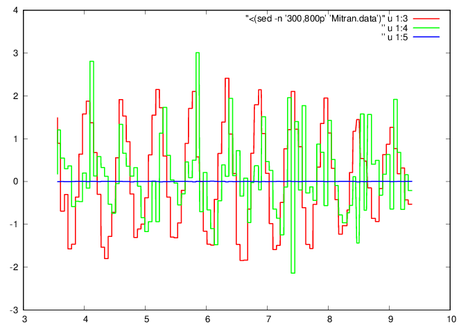
In addition to the overall plot, it is useful to plot smaller time windows

GNUplot]

cd '/home/student/courses/MATH590/NUMdata'

set terminal postscript eps enhanced color

set style line 1 lt 2 lc rgb "red" lw 3

set style line 2 lt 2 lc rgb "green" lw 3

set style line 3 lt 2 lc rgb "blue" lw 3

plot "<(sed -n '300,800p' 'Mitran.data')" u 1:3 w l ls 1, ” u 1:4 w l ls 2, ” u 1:5 w l ls 3

GNUplot]

It is remarkable that a clear waveform appears in the data. The wave form along $𝒖_{1}$ corresponds to left-right accelerations during bipedal walking. The wave form along $𝒖_{2}$ corresponds to up-down accelerations.

2.2.2Angular accelerations

GNUplot]

cd '/home/student/courses/MATH590/NUMdata'

set terminal postscript eps enhanced color

set style line 1 lt 2 lc rgb "red" lw 3

set style line 2 lt 2 lc rgb "green" lw 3

set style line 3 lt 2 lc rgb "blue" lw 3

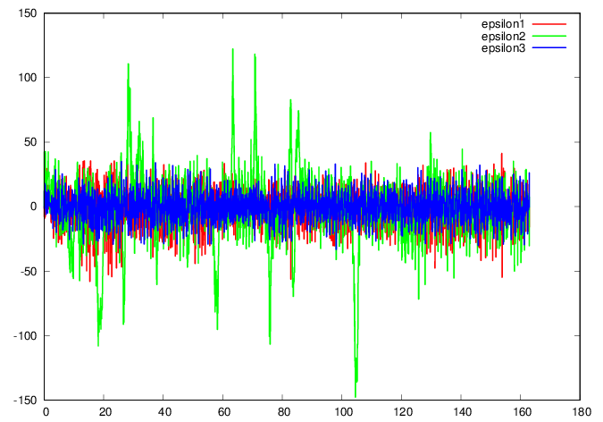
plot 'Mitran.data' u 1:5 w l ls 1 title "epsilon1", ” u 1:6 w l ls 2 title "epsilon2", ” u 1:7 w l ls 3 title "epsilon3"

GNUplot]

Observations:

There are bursts of large angular accelerations around the $𝒖_{2}$ axis. As will be seen later, this generally corresponds to the vertical axis and the bursts correspond to turns in direction of the walker.

3Trajectory reconstruction

3.1Integration

3.1.1Reconstructing angular velocities from gyroscope measurements

Recall that the integration

𝝎 (t) = \int_{0}^{t} 𝜺 (τ) d τ \Rightarrow 𝝎_{i} = 𝝎 (t_{i}) = \sum_{j = 1}^{i - 1} h_{j} 𝜺_{j}, h_{j} = t_{j + 1} - t_{j}

is essentially a non-compressive data transformation. The above is a cummulative sum, readily evaluated in Octave

octave>

shift([1 2 3 4],-1)

$(\begin{array}{cccc} 2 & 3 & 4 & 1 \end{array})$

octave>

omega=zeros([mu,3]);

h = shift(t,-1)-t;

octave>

[h(1:10) t(1:10)]

$(\begin{array}{cc} 0.004 & 0 \\ 0.001 & 0.004 \\ 0.001 & 0.005 \\ 0.001 & 0.006 \\ 0.018 & 0.007 \\ 0.031 & 0.025 \\ 0.012 & 0.056 \\ 0.033 & 0.068 \\ 0.018 & 0.101 \\ 0.001 & 0.119 \end{array})$

octave>

omega(2:mu,1) = cumsum(h(1:mu-1).*epsilon(1:mu-1,1));

omega(2:mu,2) = cumsum(h(1:mu-1).*epsilon(1:mu-1,2));

omega(2:mu,3) = cumsum(h(1:mu-1).*epsilon(1:mu-1,3));

octave>

[omega(1:6,1) epsilon(1:6,1)]

$(\begin{array}{cc} 0 & 0 \\ 0 & - 8.0329 \\ - 0.0080329 & 0.085944 \\ - 0.0079469 & 0.085944 \\ - 0.007861 & - 0.017189 \\ - 0.0081704 & - 0.017189 \end{array})$

octave>

3.1.2Reconstructing the relative coordinate system basis

The same procedure can be used to compute the time history of the relative reference frame orientation $𝐔 (t)$

\dot{𝐔} = (\begin{array}{lll} 0 & - ω_{3} & ω_{2} \\ ω_{3} & 0 & - ω_{1} \\ - ω_{2} & ω_{1} & 0 \end{array}) 𝐔 = 𝐒 𝐔 \Rightarrow 𝐔 (t_{i}) = \sum_{j = 1}^{i - 1} h_{j} 𝐒_{j} 𝐔_{j}

octave>

U=zeros([mu,3,3]); I3=eye(3); U(1,:,:)=I3; U0=I3;

octave>

i=1; while(i<mu)

om(1:3) = omega(i,1:3);

S=[0 -om(3) om(2); om(3) 0 -om(1); -om(2) om(1) 0];

[U1,R1] = qr((I3 + h(i)*S)*U0);

U1 = U1*diag(sign(diag(R1)));

U(i+1,:,:)=U1;

i++; U0=U1;

endwhile

$14189$

octave>

Display of successive $𝐔 (t_{i})$ clearly shows the rotation of the axes carried by the cell phone

octave>

i=1; di=50; while(i<300)

U1=reshape(U(i,:,:),3,3);

disp(strcat('At time t=',num2str(t(i)))); disp(U1); disp(' ');

i=i+di;

endwhile

At time t=0

   1   0   0
   0   1   0
   0   0   1
 
At time t=0.671
   0.815161  -0.376014   0.440596
   0.080612   0.826896   0.556548
  -0.573597  -0.418159   0.704365
 
At time t=1.266
   0.110337  -0.982359   0.150984
   0.200490   0.170788   0.964694
  -0.973463  -0.076171   0.215797
 
At time t=1.858
   0.675025  -0.721612   0.153679
   0.049460   0.252085   0.966440
  -0.736135  -0.644770   0.205855
 
At time t=2.502
  -0.96946  -0.20458   0.13529
   0.16788  -0.15139   0.97411
  -0.17880   0.96707   0.18111
 
At time t=3.062
  -0.385709   0.914210   0.124289
  -0.080865  -0.167693   0.982517
   0.919070   0.368915   0.138608

$1$

octave>

3.1.3Reconstructing the walker velocity and position

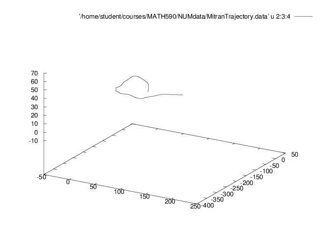
Integration of $\dot{𝑽} = 𝐔 𝒂$ and $\dot{𝑿} = 𝑽$ provides the walker trajectory

octave>

V=zeros([mu,3]); X=V; I3=eye(3); U(1,:,:)=I3; U0=I3;

octave>

i=1; while(i<mu)

U1=reshape(U(i+1,:,:),3,3);

V(i+1,:) = V(i,:) + h(i)*a(i+1,:)*U1';

X(i+1,:) = X(i,:) + h(i)*V(i+1,:);

i++;

endwhile

$14189$

octave>

Write the resulting positions and velocities to a file in preparation for plotting

octave>

fid=fopen('MitranTrajectory.data','w');

fprintf(fid,'%f %f %f %f %f %f %f\n',[t X V]');

fclose(fid);

octave>

Plot the trajectory

GNUplot]

splot '/home/student/courses/MATH590/NUMdata/MitranTrajectory.data' u 2:3:4 w l

GNUplot]

4Trajectory analysis

After reconstructing the trajectory from accelerometer data, the problem of extracting individual walker features from the data is considered.

4.1Interpolation

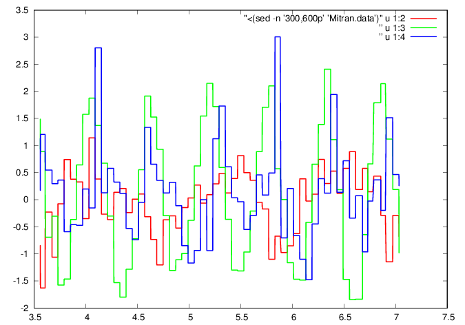
Recall that a regular pattern is apparent in the accelerometer data, one that we associate with the walker's gait. We now consider the problem of characterizing the gait

GNUplot]

cd '/home/student/courses/MATH590/NUMdata'

set terminal postscript eps enhanced color

set style line 1 lt 2 lc rgb "red" lw 3

set style line 2 lt 2 lc rgb "green" lw 3

set style line 3 lt 2 lc rgb "blue" lw 3

plot "<(sed -n '300,600p' 'Mitran.data')" u 1:2 w l ls 1, ” u 1:3 w l ls 2, ” u 1:4 w l ls 3

GNUplot]

Extract a data window of interest

octave>

iG0=300; nG=256; iG1=iG0+nG-1;

octave>

tG=t(iG0:iG1); aG=a(iG0:iG1,:);

octave>

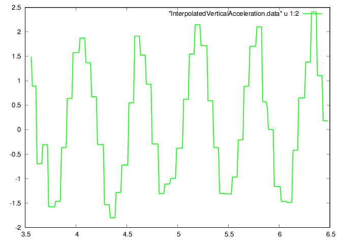
Interpolate to obtain data at constant-spaced time increments. The second component of the acceleration vector, corresponding to vertical motion is chosen (green line in above plot).

octave>

tG0=tG(1); tG1=tG(nG); dt=(tG1-tG0)/nG;

octave>

tGi=tG0+(0:nG-1)*dt;

octave>

aGi=interp1(tG',aG(:,2)',tGi);

octave>

fid=fopen('InterpolatedVerticalAcceleration.data','w');

ta = [tGi' aGi'];

fprintf(fid,'%f %f\n',ta');

fclose(fid);

octave>

Plot the interpolated data

GNUplot]

cd '/home/student/courses/MATH590/NUMdata'

set terminal postscript eps enhanced color

set style line 1 lt 2 lc rgb "green" lw 3

plot "InterpolatedVerticalAcceleration.data" u 1:2 w l ls 1

GNUplot]

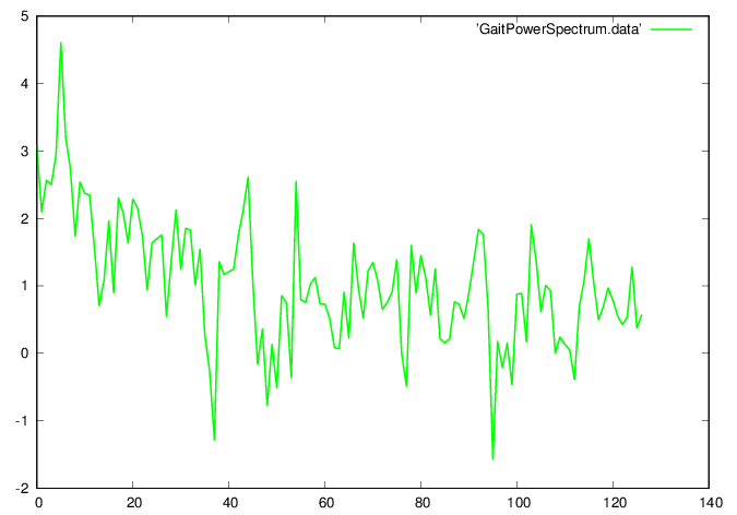
Find the period by Fourier analysis

octave>

AGi=fft(aGi); PAGi = log10(AGi.*conj(AGi));

octave>

fid=fopen('GaitPowerSpectrum.data','w');

fprintf(fid,'%f\n',PAGi(1:nG/2-1));

fclose(fid);

octave>

A plot of the power spectrum (in logarithmic coordinates) shows a distinct maximum

GNUplot]

cd '/home/student/courses/MATH590/NUMdata'

set terminal postscript eps enhanced color

set style line 1 lt 2 lc rgb "green" lw 3

plot 'GaitPowerSpectrum.data' w l ls 1

GNUplot]

octave>

[val,idx] = max(PAGi); disp([val idx]);

4.6046 6.0000

octave>

Determine the period

octave>

TG = (tG1-tG0)/(idx-1)

$0.5862$

octave>

nT=floor(max(size(aGi))/(idx-1))

$51$

octave>

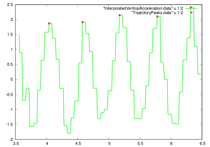
Determine locations of the peak vertical accelerations. Note that the particular values for MinPeakHeight, MinPeakDistance have to be determined by experimentation, checking the plot to see the peaks have been identified.

octave>

[aPeak, iPeak] = findpeaks(aGi-min(aGi),"MinPeakHeight",1.,"MinPeakDistance",nT/3);

fid=fopen('TrajectoryPeaks.data','w');

ta = [tGi(iPeak)' (aPeak+min(aGi))'];

fprintf(fid,'%f %f\n',ta');

fclose(fid);

octave>

nPeriods = max(size(iPeak))-1

$4$

octave>

iPeak

$(\begin{array}{ccccc} 43 & 90 & 142 & 195 & 242 \end{array})$

octave>

shift(iPeak,-1)

$(\begin{array}{ccccc} 90 & 142 & 195 & 242 & 43 \end{array})$

octave>

GNUplot]

cd '/home/student/courses/MATH590/NUMdata'

set terminal postscript eps enhanced color

set style line 1 lt 2 lc rgb "red" lw 3

set style line 2 lt 2 lc rgb "green" lw 3

set style line 3 lt 2 lc rgb "blue" lw 3

plot "InterpolatedVerticalAcceleration.data" u 1:2 w l ls 2, "TrajectoryPeaks.data" u 1:2 w p ls 1

GNUplot]

Extract data during nPeriods

First find the maximum number of data points between the maxima, allocate space for the data, and extract the measured cycles

octave>

nT = (shift(iPeak,-1)-iPeak+1)(1:nPeriods)

$(\begin{array}{cccc} 48 & 53 & 54 & 48 \end{array})$

octave>

nTmax = max(nT);

tT = zeros([nTmax,nPeriods]);

aT = zeros([nTmax,nPeriods]);

TT = zeros([nPeriods,1]);

i=1; while(i<=nPeriods)

tT(1:nT(i),i) = tGi(iPeak(i):iPeak(i+1));

aT(1:nT(i),i) = aGi(iPeak(i):iPeak(i+1));

TT(i) = tT(nT(i),i) - tT(1,i);

i++;

endwhile;

disp(TT');

0.53811 0.59536 0.60681 0.53811

octave>

Scale the data to have the same amplitude and period

octave>

i=1; while(i<=nPeriods)

tT(1:nT(i),i) = tT(1:nT(i),i) - tT(1,i);

tT(1:nT(i),i) = tT(1:nT(i),i)/TT(i);

amp = max(aT(1:nT(i),i)) - min(aT(1:nT(i),i));

aT(1:nT(i),i) = aT(1:nT(i),i)/amp;

i++;

endwhile;

octave>

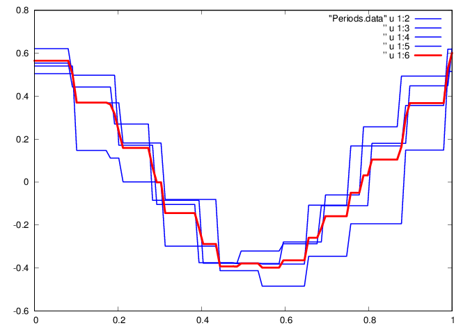
Interpolate to obtain periods with equal number of samples, and also define an average waveform $𝐠$ over the periods

octave>

nTi=100;

dt=1./(nTi-1); ti=(0:nTi-1)*dt; ti=ti';

aTi=zeros([nTi,nPeriods]); g=zeros([nTi,1]);

i=1; while(i<=nPeriods)

ai = interp1(tT(1:nT(i),i),aT(1:nT(i),i),ti',"nearest");

aTi(:,i) = ai;

g = g + ai';

i++;

endwhile;

g = g/nPeriods;

g = g/(max(g)-min(g));

octave>

fid=fopen('Periods.data','w');

ta = [ti aTi g];

fprintf(fid,'%f %f %f %f %f %f\n',ta');

fclose(fid);

fid=fopen('AveragePeriod.data','w');

ta = [ti g];

fprintf(fid,'%f %f \n',ta');

fclose(fid);

octave>

GNUplot]

cd '/home/student/courses/MATH590/NUMdata'

set terminal postscript eps enhanced color

set style line 1 lt 2 lc rgb "red" lw 6

set style line 2 lt 2 lc rgb "green" lw 3

set style line 3 lt 2 lc rgb "blue" lw 3

plot "Periods.data" u 1:2 w l ls 3, ” u 1:3 w l ls 3, ” u 1:4 w l ls 3, ” u 1:5 w l ls 3, ” u 1:6 w l ls 1

GNUplot]

4.2Least squares

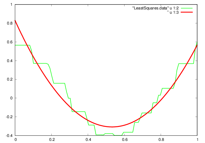
Seek a more economical representation of the average gait waveform, currently stored as a vector $𝐠 \in ℝ^{m}$ of the vertical acceleration values at times within the vector $𝐭 \in ℝ^{m}$ . For example, consider approximating the waveform by a parabola $p (t) = c_{0} + c_{1} t + c_{2} t^{2}$ , leading to the least squares problem

{min}_{𝐜 \in ℝ^{3}} || 𝐋 𝐜 - 𝐠 ||, 𝐋 = (\begin{array}{lll} 𝟏 & 𝐭 & 𝐭^{2} \end{array}) \in ℝ^{m \times 3}, 𝐭^{k} = {(\begin{array}{lll} t_{1}^{k} & \dots & t_{m}^{k} \end{array})}^{T} .

(11)

A solution is found by projection onto the column space of $𝐋$ ,

𝐐 𝐑 = 𝐋, 𝐏_{C (𝐋)} = 𝐐 𝐐^{T}, 𝐏_{C (𝐋)} 𝐠 = 𝐐 𝐑 𝐜 \Rightarrow 𝐑 𝐜 = 𝐐^{T} 𝐠 .

(12)

octave>

L=[ti.^0 ti ti.^2]; [Q,R]=qr(L,0); [size(Q); size(R)]

$(\begin{array}{cc} 100 & 3 \\ 3 & 3 \end{array})$

octave>

c = R \ Q'*g

$(\begin{array}{c} 0.82834 \\ - 4.2652 \\ 4.003 \end{array})$

octave>

p = L*c;

fid=fopen('LeastSquares.data','w');

ta = [ti g p];

fprintf(fid,'%f %f %f\n',ta');

fclose(fid);

octave>

GNUplot]

cd '/home/student/courses/MATH590/NUMdata'

set terminal postscript eps enhanced color

set style line 1 lt 2 lc rgb "red" lw 6

set style line 2 lt 2 lc rgb "green" lw 3

set style line 3 lt 2 lc rgb "blue" lw 3

plot "LeastSquares.data" u 1:2 w l ls 2, ” u 1:3 w l ls 1

GNUplot]

4.3Min-max

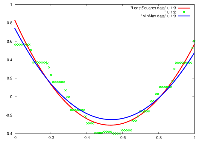
An alternative representation is through a linear combination of Chebyshev polynomials,

q (t) = d_{0} T_{0} (t) + d_{1} T_{1} (t) + d_{2} T_{2} (t)

known to be a good approximation of the min-max polynomial of the data. The coefficient vector $𝐝 \in ℝ^{3}$ is more difficult to find by comparison to the least squares case, and is carried out through a procedure known as the exchange algorithm, implemented in Octave by the polyfitinf function.

octave>

d=polyfitinf(2,nTi,0,ti,g,5.0E-7,nTi)

$(\begin{array}{ccc} 3.3996 & - 3.665 & 0.74003 \end{array})$

octave>

q = polyval(d,ti);

fid=fopen('MinMax.data','w');

ta = [ti g q];

fprintf(fid,'%f %f %f\n',ta');

fclose(fid);

octave>

GNUplot]

cd '/home/student/courses/MATH590/NUMdata'

set terminal postscript eps enhanced color

set style line 1 lt 2 lc rgb "red" lw 6

set style line 2 lt 2 lc rgb "green" lw 3

set style line 3 lt 2 lc rgb "blue" lw 6

plot "LeastSquares.data" u 1:3 w l ls 1, ” u 1:2 w p ls 2, "MinMax.data" u 1:3 w l ls 3

GNUplot]

Table of contents

1 Kinematics of rigid body motion

1.1Reference frames

1.2Matrix representation of rotations

1.3Matrix representation of infinitesimal rotations in relative coordinate system

1.4Change in the orientation of the relative coordinate system

1.5Change in position of the relative coordinate system

2Qualitative data analysis

2.1Data input

2.2Data plotting

2.2.1Linear accelerations

2.2.2Angular accelerations

3Trajectory reconstruction

3.1Integration

3.1.1Reconstructing angular velocities from gyroscope measurements

3.1.2Reconstructing the relative coordinate system basis

3.1.3Reconstructing the walker velocity and position

4Trajectory analysis

4.1Interpolation

4.2Least squares

4.3Min-max