MATH590

MATH590: Approximation in $ℝ^{d}$

Abstract

The methods of linear algebra are used to distinguish between different gaits.

1 Karhunen-Loève theorem ?

2Singular-value decomposition ?

3Covariance matrices ?

4Data-driven bases ?

5Application to gait analysis ?

1Karhunen-Loève theorem

A probability space is a triplet $(Ω, ℱ, P)$ with:

$Ω$ a sample space of all possible outcomes;
$ℱ$ a set of events that is a set of subsets of $Ω$ ;
$P : ℱ \to ℝ$ a probability function for each event.

Rather improperly named, a random variable $X : Ω \to E$ , is a function defined on a sample space with values in a measurable space (e.g., $ℝ^{d}$ ). For some measurable subset $S \subseteq E$ , the probability of $X \in S$ is

\Pr (X \in S) = P ({ω \in Ω | X (ω) \in S .})

A stochastic process $X_{t} (ω)$ is indexed collection of random variables. Often the index is time, and $X_{t} : ℝ \times Ω \to E$ . A centered stochastic process has mean value zero

𝔼 [X_{t} (ω)] = 0,

with $𝔼$ the expectation operator.

The Karhunen-Loève theorem affirms the existence of a canonical description of a stochastic process as a linear combination of random variables $Z_{k}$ with time-dependent coefficients $e_{k} (t)$ , or, conversely, as a linear combination of time-varying functions $e_{k} (t)$ with random coefficients $Z_{k}$

X_{t} (ω) = X (t, ω) = \sum_{k = 1}^{\infty} Z_{k} e_{k} (t) .

2Singular-value decomposition

As will be explained in detail in the STC module, the singular value decomposition is a discrete form of the Karhunen-Loève theorem. Let the matrix $𝐗$ denote multiple samples of some real-valued, centered stochastic process

𝐗 = (\begin{array}{llll} X (t_{1}, ω_{1}) & X (t_{1}, ω_{2}) & \dots & X (t_{1}, ω_{N}) \\ X (t_{2}, ω_{1}) & X (t_{2}, ω_{2}) & \dots & X (t_{2}, ω_{N}) \\ ⋮ & ⋮ & ⋱ & ⋮ \\ X (t_{m}, ω_{1}) & X (t_{m}, ω_{2}) & \dots & X (t_{m}, ω_{N}) \end{array}) \in ℝ^{m \times N} .

There exist orthogonal matrices $𝐔 \in ℝ^{m \times m}$ , $𝐕 \in ℝ^{N \times N}$ , and the quasi-diagonal positive matrix $𝚺 = diag (σ_{1}, \dots, σ_{r}, 0, \dots, 0) \in ℝ_{+}^{m \times N}$ such that

𝐗 = 𝐔 𝚺 𝐕^{T},

known as the singular value decomposition (SVD). Introducing the column vectors of $𝐔, 𝐕$

𝐔 = (\begin{array}{llll} 𝐮_{1} & 𝐮_{2} & \dots & 𝐮_{m} \end{array}), 𝐕 = (\begin{array}{llll} 𝐯_{1} & 𝐯_{2} & \dots & 𝐯_{N} \end{array}),

the SVD can be rewritten in two important forms:

Sum of rank-1 updates: $𝐗 = \sum_{k = 1}^{r} σ_{k} 𝐮_{k} 𝐯_{k}^{T}$
Bases for linear operator $𝐗$

3Covariance matrices

The covariance of two centered random variables $X (t_{i}, ω) = X_{i}, X (t_{j}, ω) = X_{j}$ is

cov [X_{i}, X_{j}] = 𝔼 [X_{i} X_{j}],

typically approximated through a statistic from $N$ observations

𝔼 [X_{i} X_{j}] = \frac{1}{N} \sum_{k = 1}^{N} X_{i} (ω_{k}) X_{j} (ω_{k})

The covariance matrix $𝐂$ of $m$ centered random variables $X (t_{1}, ω), \dots, X (t_{m}, ω)$ has entries

C_{i j} = cov [X_{i}, X_{j}],

and is expressed as the matrix product

𝐂 = \frac{1}{N} 𝐗 𝐗^{T} \in ℝ^{m \times m} .

By construction the covariance matrix is symmetric positive definite (spd) and therefore admits an orthogonal eigendecomposition

𝐂 = 𝐔 𝚲 𝐔^{T} = \sum_{k = 1}^{m} λ_{k} 𝐮_{k} 𝐮_{k}^{T} .

Assume (by re-labeling if necessary) that $λ_{1} ⩾ λ_{2} ⩾ \dots ⩾ λ_{m}$ . It is often the case that $p$ eigenvalues dominate over all others (the strongly correlated modes)

λ_{1} ⩾ λ_{2} ⩾ \dots ⩾ λ_{p} ≫ λ_{p + 1} ⩾ \dots ⩾ λ_{m},

and the correlation matrix is approximated by the first $p$ rank-1 updates

𝐂 ≅ \sum_{k = 1}^{p} λ_{k} 𝐮_{k} 𝐮_{k}^{T} .

4Data-driven bases

The dominant correlated modes form a natural basis set for analysis of data. Rather than solving the covariance matrix eigenproblem the SVD of $𝐗$ is used since

𝐗 = 𝐔 𝚺 𝐕^{T}, N 𝐂 = 𝐗 𝐗^{T} = 𝐔 𝚺 𝐕^{T} 𝐕 𝚺^{T} 𝐔^{T} = 𝐔 𝚺 𝚺^{T} 𝐔^{T} .

5Application to gait analysis

Consider the data obtained from many individual gait measurements (either from different individuals or at different times for the same individual). The goal is to identify differences w.r.t. a mean gait and use those differences to (1) identify either an individual or (2) a particular type of walking (climbing stairs versus level walking). The procedure is demonstrated here for the second problem.

octave>

dir='/home/student/courses/MATH590/NUMdata';

chdir(dir);

LastName='Mitran';

d=textread(strcat(LastName,'.data'));

mu=max(size(d))/7; disp(mu)

14190

/home/student/courses/MATH590/NUMdata

octave>

data=reshape(d,[7,mu])';

data(1:6,1:7)

$(\begin{array}{ccccccc} 0 & 0 & 0 & 0 & 0 & 0 & 0 \\ 0.004 & - 0.7803 & 0.2999 & - 1.799 & - 8.0329 & 16.868 & 3.0539 \\ 0.005 & - 0.0953 & 0.0762 & - 0.0111 & 0.085944 & 21.033 & 12.152 \\ 0.006 & - 0.0953 & 0.0762 & - 0.0111 & 0.085944 & 21.033 & 12.152 \\ 0.007 & - 0.6242 & - 0.0203 & - 0.9742 & - 0.017189 & 42.279 & - 1.5986 \\ 0.025 & - 0.6242 & - 0.0203 & - 0.9742 & - 0.017189 & 42.279 & - 1.5986 \end{array})$

octave>

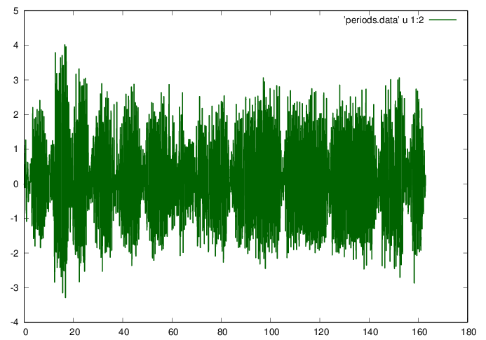
Interpolate to obtain even-spaced data, and plot the data.

octave>

t0=data(1,1); t1=data(mu,1); ni = 2^ceil(log2(mu)); dt=(t1-t0)/ni;

ti=(0:ni-1)*dt; ti=ti';

ai=interp1(data(:,1),data(:,3),ti);

fid=fopen('periods.data','w');

fprintf(fid,'%f %f\n',[ti ai]');

fclose(fid);

octave>

GNUplot]

cd '/home/student/courses/MATH590/NUMdata'

set terminal postscript eps enhanced color

set style line 1 lt 2 lc rgb "0x00006400" lw 3

plot 'periods.data' u 1:2 w l ls 1

GNUplot]

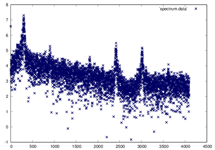
Find the Fourier spectrum of the vertical acceleration data.

octave>

Ai=fft(ai); PAi=log10(Ai.*conj(Ai));

fid=fopen('spectrum.data','w');

fprintf(fid,'%f\n',PAi(1:ni/4));

fclose(fid);

octave>

GNUplot]

cd '/home/student/courses/MATH590/NUMdata'

set terminal postscript eps enhanced color

set style line 1 lt 2 lc rgb "0x00000064" lw 3

plot 'spectrum.data' ls 1

GNUplot]

There are several peaks within the Fourier spectrum. Seek the peak corresponding to a natural step period of approximately $T_{s} = (t_{1} - t_{0}) / n_{Steps} ≅ 0.5 s$ . This turns out to be close to the global peak as shown in the following calculations

octave>

ks=floor((t1-t0)/(0.5))

$325$

octave>

[PAimx imx]=max(PAi);

octave>

[PAimx imx]

$(\begin{array}{cc} 7.3053 & 299 \end{array})$

octave>

N=imx-1;

octave>

Ts=(t1-t0)/N

$0.54679$

octave>

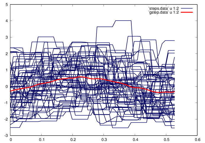
Isolate the steps, find an average step waveform $g$ , and compute the centered data matrix $𝐗$

octave>

m = floor(ni/N); t=(0:m-1)'*dt;

a = reshape(ai(2:m*N+1),[m,N]); g = mean(a')';

X = a - repmat(g,1,N);

octave>

fid=fopen('steps.data','w');

i=1; while(i<N)

fprintf(fid,'%f %f\n',[t a(:,i)]');

fprintf(fid,'\n');

i=i+5;

endwhile;

fclose(fid);

octave>

fid=fopen('gstep.data','w');

fprintf(fid,'%f %f\n',[t g]');

fclose(fid);

octave>

GNUplot]

cd '/home/student/courses/MATH590/NUMdata'

set terminal postscript eps enhanced color

set style line 1 lt 2 lc rgb "0x00000064" lw 3

set style line 2 lt 2 lc rgb "0x00ff0000" lw 6

plot 'steps.data' u 1:2 w l ls 1, 'gstep.data' u 1:2 w l ls 2

GNUplot]

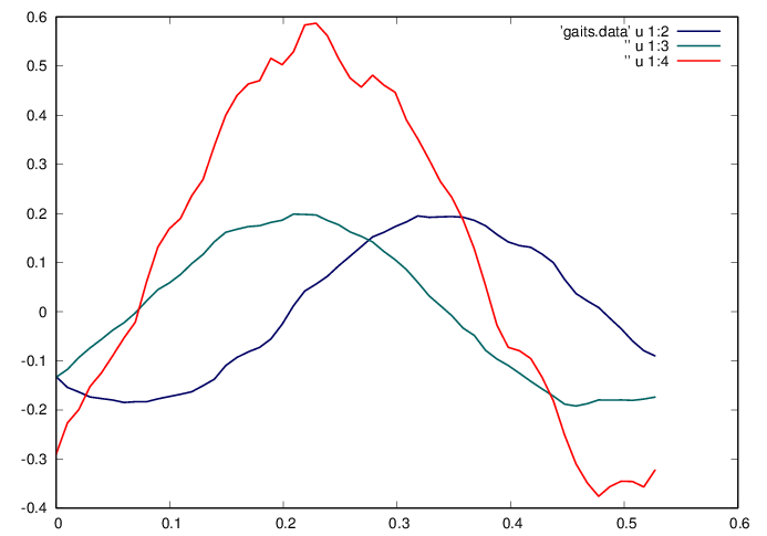
Find the natural basis for the problem by computing the SVD of $𝐗$ , and investigate the dominant singular values

octave>

[U,S,V]=svd(X,0);

octave>

(diag(S)(1:6))'

$(\begin{array}{cccccc} 108.031 & 93.528 & 23.645 & 19.604 & 17.588 & 15.726 \end{array})$

octave>

fid=fopen('gaits.data','w');

fprintf(fid,'%f %f %f %f\n',[t U(:,1:2) g]');

fclose(fid);

octave>

From the above each step can be characterized by the first two components $𝐮_{1}, 𝐮_{2}$ . Plot these modes and compare to the average gait $𝐠$ .

GNUplot]

cd '/home/student/courses/MATH590/NUMdata'

set terminal postscript eps enhanced color

set style line 1 lt 2 lc rgb "0x00000064" lw 3

set style line 2 lt 2 lc rgb "0x00006464" lw 3

set style line 3 lt 2 lc rgb "0x00FF0000" lw 3

plot 'gaits.data' u 1:2 w l ls 1, ” u 1:3 w l ls 2, ” u 1:4 w l ls 3

GNUplot]

Find the coordinates $𝐜$ of each step along these directions.

octave>

c=X'*U(:,1:2);

fid=fopen('coefs.data','w');

fprintf(fid,'%f %f\n',c');

fclose(fid);

octave>

size(c)

$(\begin{array}{cc} 298 & 2 \end{array})$

octave>

GNUplot]

cd '/home/student/courses/MATH590/NUMdata'

set terminal postscript eps enhanced color

set style line 1 lt 2 lc rgb "0x00000064" lw 3

plot 'coefs.data' u 1:2 w p ls 1

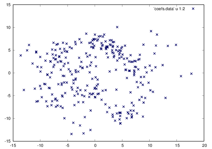
GNUplot]

At this point, an economical representation of each of the $N$ steps has been obtained, and the next question is to classify the observed results. This forms the objective of clustering analysis that relies on the mathematical theory of sets, as presented in the next module.

Table of contents

1Karhunen-Loève theorem

2Singular-value decomposition

3Covariance matrices

4Data-driven bases

5Application to gait analysis