MATH590

MATH590 Homework 1: Approximation in $ℝ^{d}$

Carry out analysis of the cell-phone accelerometer data according to the following template, answering the questions. The objective of this homework is to familiarize yourself with some linear algebra and numerical analysis techniques that are commonly encountered in data analysis.

Turn in this TeXmacs file and the two data files AveragePeriod.LastName.data, PolyCoef.LastName.data. The results contained in these files will be used in subsequent topological data analysis.

1Qualitative data analysis

A first step in processing the data $(𝒂, 𝜺)$ acquired from the cell phone is to carry out some basic qualitative analysis, shown here using Octave (Matlab clone).

1.1Data input

1.1.1Visual inspection of data

octave>

dir='/home/student/courses/MATH590/NUMdata';

chdir(dir);

LastName = 'Mitran';

data=csvread(strcat(LastName,'.csv'));

[m,d] = size(data); disp([m d]);

18841 8

octave>

data(1:30,:)

$(\begin{array}{cccccccc} 0 & 0 & 0 & 0 & 0 & 0 & 0 & 0 \\ 0.004 & - 0.7803 & 0.2999 & - 1.799 & - 0.1402 & 0.2944 & 0.0533 & 0 \\ 0.005 & - 0.7803 & 0.2999 & - 1.799 & 0.0015 & 0.3671 & 0.2121 & 0 \\ 0.005 & - 0.0953 & 0.0762 & - 0.0111 & 0.0015 & 0.3671 & 0.2121 & 0 \\ 0.006 & - 0.0953 & 0.0762 & - 0.0111 & 0.0015 & 0.3671 & 0.2121 & 0 \\ 0.006 & - 0.0953 & 0.0762 & - 0.0111 & 0.0015 & 0.3671 & 0.2121 & 0 \\ 0.006 & - 0.0953 & 0.0762 & - 0.0111 & 0.0015 & 0.3671 & 0.2121 & 0 \\ 0.006 & - 0.0953 & 0.0762 & - 0.0111 & 0.0015 & 0.3671 & 0.2121 & 0 \\ 0.006 & - 0.0953 & 0.0762 & - 0.0111 & 0.0015 & 0.3671 & 0.2121 & 0 \\ 0.007 & - 0.0953 & 0.0762 & - 0.0111 & - 0.0003 & 0.7379 & - 0.0279 & 0 \\ 0.007 & - 0.6242 & - 0.0203 & - 0.9742 & - 0.0003 & 0.7379 & - 0.0279 & 0 \\ 0.025 & - 0.6242 & - 0.0203 & - 0.9742 & - 0.0003 & 0.7379 & - 0.0279 & 0 \\ 0.056 & - 0.6242 & - 0.0203 & - 0.9742 & - 0.0003 & 0.7379 & - 0.0279 & 0 \\ 0.056 & - 0.6242 & - 0.0203 & - 0.9742 & - 0.0003 & 0.7379 & - 0.0279 & 0 \\ 0.056 & - 0.6242 & - 0.0203 & - 0.9742 & - 0.0003 & 0.7379 & - 0.0279 & 0 \\ 0.068 & - 0.6242 & - 0.0203 & - 0.9742 & - 0.0003 & 0.7379 & - 0.0279 & 0 \\ 0.068 & - 0.6242 & - 0.0203 & - 0.9742 & - 0.1671 & 0.3402 & 0.2799 & 0 \\ 0.068 & - 1.0653 & 0.5028 & - 0.6942 & - 0.1671 & 0.3402 & 0.2799 & 0 \\ 0.101 & - 1.0653 & 0.5028 & - 0.6942 & - 0.1671 & 0.3402 & 0.2799 & 0 \\ 0.119 & - 1.0653 & 0.5028 & - 0.6942 & - 0.1671 & 0.3402 & 0.2799 & 0 \\ 0.12 & - 1.0653 & 0.5028 & - 0.6942 & - 0.1671 & 0.3402 & 0.2799 & 0 \\ 0.12 & - 1.0653 & 0.5028 & - 0.6942 & - 0.1671 & 0.3402 & 0.2799 & 0 \\ 0.126 & - 1.0653 & 0.5028 & - 0.6942 & - 0.1671 & 0.3402 & 0.2799 & 0 \\ 0.126 & - 1.0653 & 0.5028 & - 0.6942 & - 0.0082 & 0.5577 & 0.2268 & 0 \\ 0.127 & - 0.1956 & 0.0971 & - 0.7178 & - 0.0082 & 0.5577 & 0.2268 & 0 \\ 0.176 & - 0.1956 & 0.0971 & - 0.7178 & - 0.0082 & 0.5577 & 0.2268 & 0 \\ 0.177 & - 0.1956 & 0.0971 & - 0.7178 & - 0.0082 & 0.5577 & 0.2268 & 0 \\ 0.177 & - 0.1956 & 0.0971 & - 0.7178 & - 0.0082 & 0.5577 & 0.2268 & 0 \\ 0.186 & - 0.1956 & 0.0971 & - 0.7178 & - 0.0082 & 0.5577 & 0.2268 & 0 \\ 0.186 & - 0.1956 & 0.0971 & - 0.7178 & - 0.1506 & 0.5546 & 0.3117 & 0 \end{array})$

octave>

Question 1.

Identify to which directions (forward walking, up and down, sideways) each column corresponds

Column Notation Physical quantity Units
1 t time s
2 $a_{1}$ sideways acceleration m/s
3 $a_{2}$ up-down acceleration m/s
4 $a_{3}$ forward-backward acceleration m/s
5 $ω_{1}$ pitch angular velocity rad/s
6 $ω_{2}$ yaw angular velocity rad/s
7 $ω_{3}$ roll angular velocity rad/s

Table 1. Data notation, significance, units

Identify the physical units used in the measurements

See Table 1.

Are the values reasonable?

One step occurs every approximately every T=0.75 seconds. During that time a person's center of gravity moves up and down by about h=0.125 m, giving upward velocity of $v_{2} = h / (T / 2) ≅ 0.3 m / s$ , $a_{2} = 2 v_{2} / T = 0.88 m / s^{2}$ , and this is the order of magnitude of the values in the $a_{3}$ column, so the values seem reasonable. Also, the sideways acceleration values are consistently smaller, and the forward values about the same as the vertical ones and, importantly, out of phase as expected in a normal gait. The largest angular velocities correspond to yaw, also as expected since this is the alternating forward-backward motion of left-right side of the body during the gait. Finally, walking is an effort against gravitational acceleration $g = 9.8 m / s^{2}$ , and one would expect values about one-tenth of $g$ .

1.1.2Plot data

Write data to a file.

octave>

[t,iu]=unique(data(:,1));

mu=max(size(iu));

raddeg=pi/180;

a=data(iu,2:4); epsilon=data(iu,5:7)/raddeg;

fid=fopen(strcat(LastName,'.data'),'w');

fprintf(fid,'%f %f %f %f %f %f %f\n',[t a epsilon]');

fclose(fid);

octave>

Change the file plotted to your data.

GNUplot]

cd '/home/student/courses/MATH590/NUMdata'

set terminal postscript eps enhanced color

set style line 1 lt 2 lc rgb "red" lw 3

set style line 2 lt 2 lc rgb "green" lw 3

set style line 3 lt 2 lc rgb "blue" lw 3

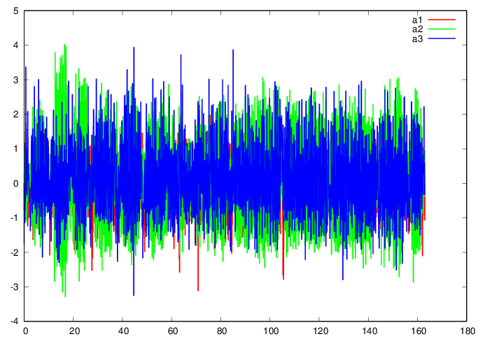
plot 'Mitran.data' u 1:2 w l ls 1 title "a1", ” u 1:3 w l ls 2 title "a2", ” u 1:4 w l ls 3 title "a3"

GNUplot]

cd '/home/student/courses/MATH590/NUMdata'

set terminal postscript eps enhanced color

set style line 1 lt 2 lc rgb "red" lw 3

set style line 2 lt 2 lc rgb "green" lw 3

set style line 3 lt 2 lc rgb "blue" lw 3

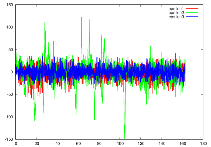
plot 'Mitran.data' u 1:5 w l ls 1 title "epsilon1", ” u 1:6 w l ls 2 title "epsilon2", ” u 1:7 w l ls 3 title "epsilon3"

GNUplot]

Question 2. What are your observations on the physical relevance of the data?

Data shows an average close to zero, as expected, with large values for yaw angular velocity in the data that appear correleated with turns in the path.

2Extract walker gait data

2.1Choose a data window

Modify the data window as needed

GNUplot]

cd '/home/student/courses/MATH590/NUMdata'

set terminal postscript eps enhanced color

set style line 1 lt 2 lc rgb "red" lw 3

set style line 2 lt 2 lc rgb "green" lw 3

set style line 3 lt 2 lc rgb "blue" lw 3

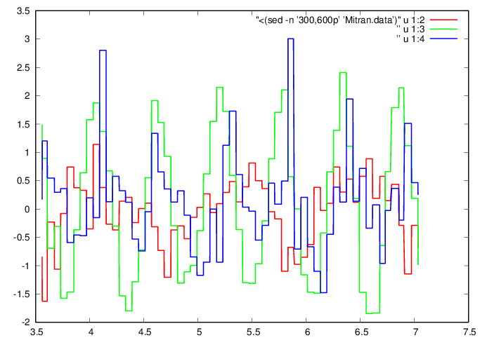
plot "<(sed -n '300,600p' 'Mitran.data')" u 1:2 w l ls 1, ” u 1:3 w l ls 2, ” u 1:4 w l ls 3

GNUplot]

octave>

iG0=300; nG=256; iG1=iG0+nG-1;

tG=t(iG0:iG1); aG=a(iG0:iG1,:);

tG0=tG(1); tG1=tG(nG); dt=(tG1-tG0)/nG;

tGi=tG0+(0:nG-1)*dt;

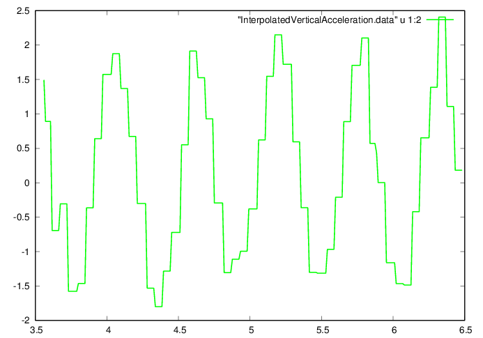
aGi=interp1(tG',aG(:,2)',tGi);

fid=fopen('InterpolatedVerticalAcceleration.data','w');

ta = [tGi' aGi'];

fprintf(fid,'%f %f\n',ta');

fclose(fid);

octave>

GNUplot]

cd '/home/student/courses/MATH590/NUMdata'

set terminal postscript eps enhanced color

set style line 1 lt 2 lc rgb "green" lw 3

plot "InterpolatedVerticalAcceleration.data" u 1:2 w l ls 1

GNUplot]

Question 3. How do you explain changes in the vertical acceleration between steps?

This is the expected acceleration of the body's center of mass during stepping motion. In contrast if this was rolling motion (i.e., on wheels) the vertical acceleration should be small. This values shows even large variation when stepping on stairs.

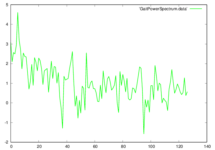
2.2Determine gait period

octave>

AGi=fft(aGi); PAGi = log10(AGi.*conj(AGi));

fid=fopen('GaitPowerSpectrum.data','w');

fprintf(fid,'%f\n',PAGi(1:nG/2-1));

fclose(fid);

octave>

GNUplot]

cd '/home/student/courses/MATH590/NUMdata'

set terminal postscript eps enhanced color

set style line 1 lt 2 lc rgb "green" lw 3

plot 'GaitPowerSpectrum.data' w l ls 1

GNUplot]

octave>

[val,idx] = max(PAGi); disp([val idx]);

4.6046 6.0000

octave>

TG = (tG1-tG0)/(idx-1)

$0.5862$

octave>

nT=floor(max(size(aGi))/(idx-1))

$51$

octave>

Question 4. Does the period value correspond to a full stride or stepping on one leg?

The period corresponds to stepping on one leg. A full stride (returning to the same foot on the ground at start of step) corresponds to 2 periods.

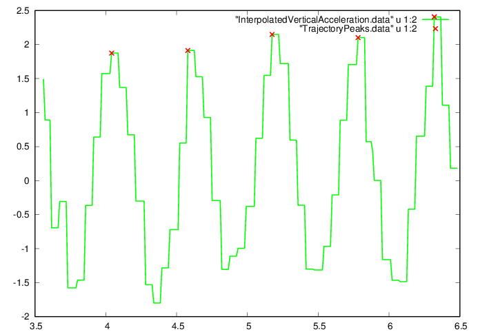
2.3Splice data into multiple periods

Find peak vertical accelerations.

octave>

[aPeak, iPeak] = findpeaks(aGi-min(aGi),"MinPeakHeight",1.,"MinPeakDistance",nT/3);

fid=fopen('TrajectoryPeaks.data','w');

ta = [tGi(iPeak)' (aPeak+min(aGi))'];

fprintf(fid,'%f %f\n',ta');

fclose(fid);

octave>

nPeriods = max(size(iPeak))-1

$4$

octave>

Plot the acceleration peaks.

GNUplot]

cd '/home/student/courses/MATH590/NUMdata'

set terminal postscript eps enhanced color

set style line 1 lt 2 lc rgb "red" lw 3

set style line 2 lt 2 lc rgb "green" lw 3

set style line 3 lt 2 lc rgb "blue" lw 3

plot "InterpolatedVerticalAcceleration.data" u 1:2 w l ls 2, "TrajectoryPeaks.data" u 1:2 w p ls 1

GNUplot]

Extract the periods

octave>

nT = (shift(iPeak,-1)-iPeak+1)(1:nPeriods)

$(\begin{array}{cccc} 48 & 53 & 54 & 48 \end{array})$

octave>

nTmax = max(nT);

tT = zeros([nTmax,nPeriods]);

aT = zeros([nTmax,nPeriods]);

TT = zeros([nPeriods,1]);

i=1; while(i<=nPeriods)

tT(1:nT(i),i) = tGi(iPeak(i):iPeak(i+1));

aT(1:nT(i),i) = aGi(iPeak(i):iPeak(i+1));

TT(i) = tT(nT(i),i) - tT(1,i);

i++;

endwhile;

disp(TT');

0.53811 0.59536 0.60681 0.53811

octave>

i=1; while(i<=nPeriods)

tT(1:nT(i),i) = tT(1:nT(i),i) - tT(1,i);

tT(1:nT(i),i) = tT(1:nT(i),i)/TT(i);

amp = max(aT(1:nT(i),i)) - min(aT(1:nT(i),i));

aT(1:nT(i),i) = aT(1:nT(i),i)/amp;

i++;

endwhile;

octave>

nTi=100;

dt=1./(nTi-1); ti=(0:nTi-1)*dt; ti=ti';

aTi=zeros([nTi,nPeriods]); g=zeros([nTi,1]);

i=1; while(i<=nPeriods)

ai = interp1(tT(1:nT(i),i),aT(1:nT(i),i),ti',"nearest");

aTi(:,i) = ai;

g = g + ai';

i++;

endwhile;

g = g/nPeriods;

g = g/(max(g)-min(g));

octave>

fid=fopen('Periods.data','w');

ta = [ti aTi g];

fprintf(fid,'%f %f %f %f %f %f\n',ta');

fclose(fid);

fid=fopen(strcat(strcat('AveragePeriod.',LastName),'.data'),'w');

ta = [ti g];

fprintf(fid,'%f %f \n',ta');

fclose(fid);

octave>

GNUplot]

cd '/home/student/courses/MATH590/NUMdata'

set terminal postscript eps enhanced color

set style line 1 lt 2 lc rgb "red" lw 6

set style line 2 lt 2 lc rgb "green" lw 3

set style line 3 lt 2 lc rgb "blue" lw 3

plot "Periods.data" u 1:2 w l ls 3, ” u 1:3 w l ls 3, ” u 1:4 w l ls 3, ” u 1:5 w l ls 3, ” u 1:6 w l ls 1

GNUplot]

Question 5. What are the potential drawbacks of defining an “average” gait? Consider the limiting cases of too few or very many sample periods.

For too many periods, differences in the path (climbing, turning, descending) can mask the average gait assumed to be specific to a person. For, say, a single period, the gait might not be typical, e.g., due to a cough or irregularity in the path. It would be best to more carefully control the path in order to identify the person, e.g., limit data to walking a straight path of 10 meters.

2.4Least squares

Seek a more economical representation of the average gait waveform, currently stored as a vector $𝐠 \in ℝ^{m}$ of the vertical acceleration values at times within the vector $𝐭 \in ℝ^{m}$ . For example, consider approximating the waveform by a parabola $p (t) = c_{0} + c_{1} t + c_{2} t^{2}$ , leading to the least squares problem

{min}_{𝐜 \in ℝ^{3}} || 𝐋 𝐜 - 𝐠 ||, 𝐋 = (\begin{array}{lll} 𝟏 & 𝐭 & 𝐭^{2} \end{array}) \in ℝ^{m \times 3}, 𝐭^{k} = {(\begin{array}{lll} t_{1}^{k} & \dots & t_{m}^{k} \end{array})}^{T} .

(1)

A solution is found by projection onto the column space of $𝐋$ ,

𝐐 𝐑 = 𝐋, 𝐏_{C (𝐋)} = 𝐐 𝐐^{T}, 𝐏_{C (𝐋)} 𝐠 = 𝐐 𝐑 𝐜 \Rightarrow 𝐑 𝐜 = 𝐐^{T} 𝐠 .

(2)

octave>

L=[ti.^0 ti ti.^2]; [Q,R]=qr(L,0); [size(Q); size(R)]

$(\begin{array}{cc} 100 & 3 \\ 3 & 3 \end{array})$

octave>

c = R \ Q'*g

$(\begin{array}{c} 0.82834 \\ - 4.2652 \\ 4.003 \end{array})$

octave>

p = L*c;

fid=fopen('LeastSquares.data','w');

ta = [ti g p];

fprintf(fid,'%f %f %f\n',ta');

fclose(fid);

octave>

GNUplot]

cd '/home/student/courses/MATH590/NUMdata'

set terminal postscript eps enhanced color

set style line 1 lt 2 lc rgb "red" lw 6

set style line 2 lt 2 lc rgb "green" lw 3

set style line 3 lt 2 lc rgb "blue" lw 3

plot "LeastSquares.data" u 1:2 w l ls 2, ” u 1:3 w l ls 1

GNUplot]

Question 6. What gait information is lost in the least squares approximation?

Think of the motion as being produced by a triple articulated structure (at knees, hips, shoulders). Through a quadratic approximation, the above are combined into a single articulation, hence the acceleration profile provided by specific lengths of shins, thighs, backbone are lost.

2.5Min-max

An alternative representation is through a linear combination of Chebyshev polynomials,

q (t) = d_{0} T_{0} (t) + d_{1} T_{1} (t) + d_{2} T_{2} (t)

known to be a good approximation of the min-max polynomial of the data. The coefficient vector $𝐝 \in ℝ^{3}$ is more difficult to find by comparison to the least squares case, and is carried out through a procedure known as the exchange algorithm, implemented in Octave by the polyfitinf function.

octave>

d=polyfitinf(2,nTi,0,ti,g,5.0E-7,nTi)

$(\begin{array}{ccc} 3.3996 & - 3.665 & 0.74003 \end{array})$

octave>

q = polyval(d,ti);

fid=fopen('MinMax.data','w');

ta = [ti g q];

fprintf(fid,'%f %f %f\n',ta');

fclose(fid);

octave>

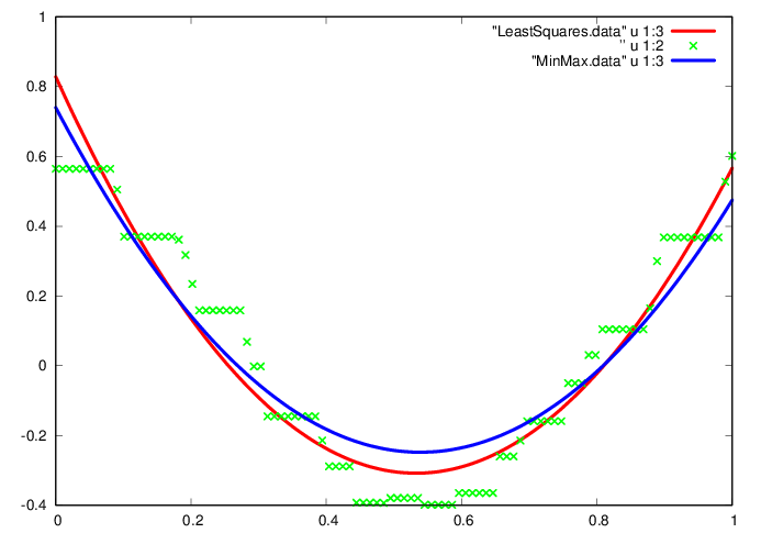
GNUplot]

cd '/home/student/courses/MATH590/NUMdata'

set terminal postscript eps enhanced color

set style line 1 lt 2 lc rgb "red" lw 6

set style line 2 lt 2 lc rgb "green" lw 3

set style line 3 lt 2 lc rgb "blue" lw 6

plot "LeastSquares.data" u 1:3 w l ls 1, ” u 1:2 w p ls 2, "MinMax.data" u 1:3 w l ls 3

GNUplot]

Question 7. Which gait approximation is better suited to walker identification, least squares or min-max? Explain your reasoning.

Min-max is suited to approximation that minimizes a presumed “maximal” error. The problem is that such a maximal error cannot be defined in this case, whereas, for example, it is straightforward to define in the approximation of an analytical function such as sin(x). The least-squares approximation is better in this case.

Save the coefficients of the two representations (least-squares and Chebyshev)

octave>

fid=fopen(strcat(strcat('PolyCoef.',LastName),'.data'),'w');

ta = [c d'];

fprintf(fid,'%f %f\n',ta');

fclose(fid);

octave>