MATH590

MATH590 Homework 1: Approximation in $ℝ^{d}$

Carry out analysis of the cell-phone accelerometer data according to the following template, answering the questions. The objective of this homework is to familiarize yourself with some linear algebra and numerical analysis techniques that are commonly encountered in data analysis.

Turn in this TeXmacs file and the two data files AveragePeriod.LastName.data, PolyCoef.LastName.data. The results contained in these files will be used in subsequent topological data analysis.

1Qualitative data analysis

A first step in processing the data $(𝒂, 𝜺)$ acquired from the cell phone is to carry out some basic qualitative analysis, shown here using Octave (Matlab clone).

1.1Data input

1.1.1Visual inspection of data

octave>

dir='/home/student/courses/MATH590/NUMdata';

chdir(dir);

LastName = 'Mitran';

data=csvread(strcat(LastName,'.csv'));

[m,d] = size(data); disp([m d]);

18841 8

octave>

data(1:10,:)

$(\begin{array}{cccccccc} 0 & 0 & 0 & 0 & 0 & 0 & 0 & 0 \\ 0.004 & - 0.7803 & 0.2999 & - 1.799 & - 0.1402 & 0.2944 & 0.0533 & 0 \\ 0.005 & - 0.7803 & 0.2999 & - 1.799 & 0.0015 & 0.3671 & 0.2121 & 0 \\ 0.005 & - 0.0953 & 0.0762 & - 0.0111 & 0.0015 & 0.3671 & 0.2121 & 0 \\ 0.006 & - 0.0953 & 0.0762 & - 0.0111 & 0.0015 & 0.3671 & 0.2121 & 0 \\ 0.006 & - 0.0953 & 0.0762 & - 0.0111 & 0.0015 & 0.3671 & 0.2121 & 0 \\ 0.006 & - 0.0953 & 0.0762 & - 0.0111 & 0.0015 & 0.3671 & 0.2121 & 0 \\ 0.006 & - 0.0953 & 0.0762 & - 0.0111 & 0.0015 & 0.3671 & 0.2121 & 0 \\ 0.006 & - 0.0953 & 0.0762 & - 0.0111 & 0.0015 & 0.3671 & 0.2121 & 0 \\ 0.007 & - 0.0953 & 0.0762 & - 0.0111 & - 0.0003 & 0.7379 & - 0.0279 & 0 \end{array})$

octave>

Question 1.

Identify to which directions (forward walking, up and down, sideways) each column corresponds

Identify the physical units used in the measurements

Are the values reasonable?

1.1.2Plot data

Write data to a file.

octave>

[t,iu]=unique(data(:,1));

mu=max(size(iu));

raddeg=pi/180;

a=data(iu,2:4); epsilon=data(iu,5:7)/raddeg;

fid=fopen(strcat(LastName,'.data'),'w');

fprintf(fid,'%f %f %f %f %f %f %f\n',[t a epsilon]');

fclose(fid);

octave>

Change the file plotted to your data.

GNUplot]

cd '/home/student/courses/MATH590/NUMdata'

set terminal postscript eps enhanced color

set style line 1 lt 2 lc rgb "red" lw 3

set style line 2 lt 2 lc rgb "green" lw 3

set style line 3 lt 2 lc rgb "blue" lw 3

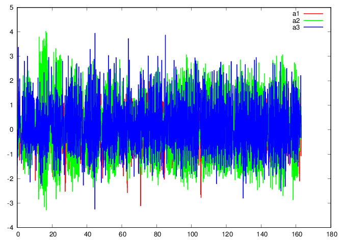
plot 'Mitran.data' u 1:2 w l ls 1 title "a1", ” u 1:3 w l ls 2 title "a2", ” u 1:4 w l ls 3 title "a3"

GNUplot]

cd '/home/student/courses/MATH590/NUMdata'

set terminal postscript eps enhanced color

set style line 1 lt 2 lc rgb "red" lw 3

set style line 2 lt 2 lc rgb "green" lw 3

set style line 3 lt 2 lc rgb "blue" lw 3

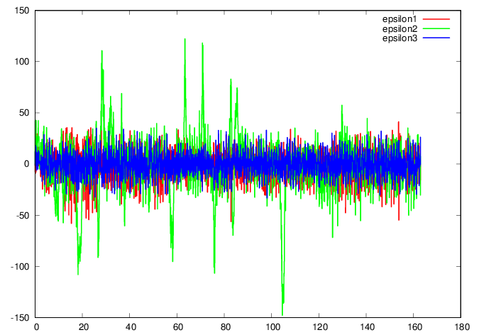
plot 'Mitran.data' u 1:5 w l ls 1 title "epsilon1", ” u 1:6 w l ls 2 title "epsilon2", ” u 1:7 w l ls 3 title "epsilon3"

GNUplot]

Question 2. What are your observations on the physical relevance of the data?

2Extract walker gait data

2.1Choose a data window

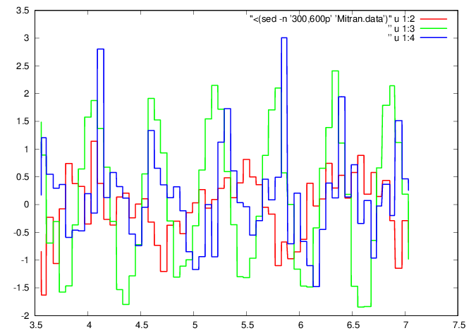
Modify the data window as needed

GNUplot]

cd '/home/student/courses/MATH590/NUMdata'

set terminal postscript eps enhanced color

set style line 1 lt 2 lc rgb "red" lw 3

set style line 2 lt 2 lc rgb "green" lw 3

set style line 3 lt 2 lc rgb "blue" lw 3

plot "<(sed -n '300,600p' 'Mitran.data')" u 1:2 w l ls 1, ” u 1:3 w l ls 2, ” u 1:4 w l ls 3

GNUplot]

octave>

iG0=300; nG=256; iG1=iG0+nG-1;

tG=t(iG0:iG1); aG=a(iG0:iG1,:);

tG0=tG(1); tG1=tG(nG); dt=(tG1-tG0)/nG;

tGi=tG0+(0:nG-1)*dt;

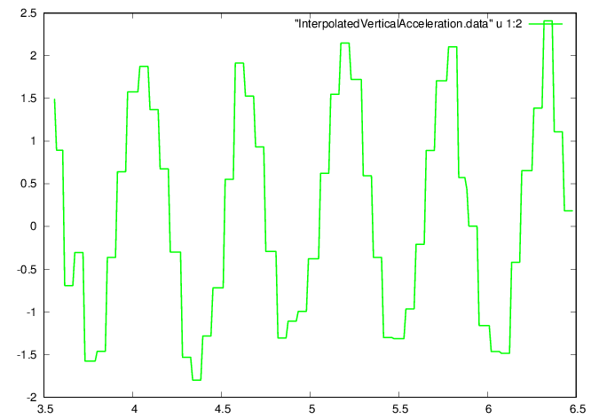
aGi=interp1(tG',aG(:,2)',tGi);

fid=fopen('InterpolatedVerticalAcceleration.data','w');

ta = [tGi' aGi'];

fprintf(fid,'%f %f\n',ta');

fclose(fid);

octave>

GNUplot]

cd '/home/student/courses/MATH590/NUMdata'

set terminal postscript eps enhanced color

set style line 1 lt 2 lc rgb "green" lw 3

plot "InterpolatedVerticalAcceleration.data" u 1:2 w l ls 1

GNUplot]

Question 3. How do you explain changes in the vertical acceleration between steps?

2.2Determine gait period

octave>

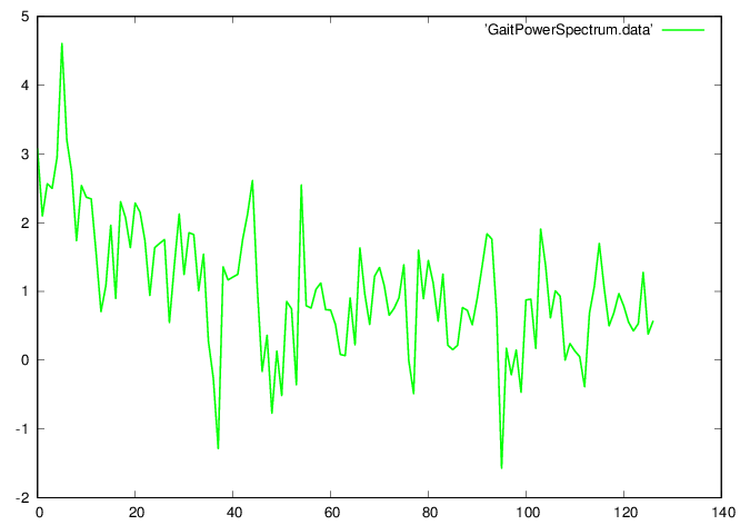
AGi=fft(aGi); PAGi = log10(AGi.*conj(AGi));

fid=fopen('GaitPowerSpectrum.data','w');

fprintf(fid,'%f\n',PAGi(1:nG/2-1));

fclose(fid);

octave>

GNUplot]

cd '/home/student/courses/MATH590/NUMdata'

set terminal postscript eps enhanced color

set style line 1 lt 2 lc rgb "green" lw 3

plot 'GaitPowerSpectrum.data' w l ls 1

GNUplot]

octave>

[val,idx] = max(PAGi); disp([val idx]);

4.6046 6.0000

octave>

TG = (tG1-tG0)/(idx-1)

$0.5862$

octave>

nT=floor(max(size(aGi))/(idx-1))

$51$

octave>

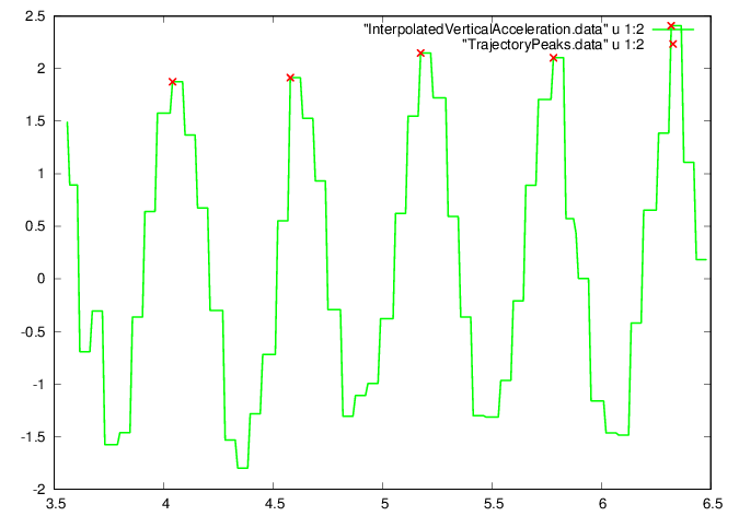
Question 4. Does the period value correspond to a full stride or stepping on one leg?

2.3Splice data into multiple periods

Find peak vertical accelerations.

octave>

[aPeak, iPeak] = findpeaks(aGi-min(aGi),"MinPeakHeight",1.,"MinPeakDistance",nT/3);

fid=fopen('TrajectoryPeaks.data','w');

ta = [tGi(iPeak)' (aPeak+min(aGi))'];

fprintf(fid,'%f %f\n',ta');

fclose(fid);

octave>

nPeriods = max(size(iPeak))-1

$4$

octave>

Plot the acceleration peaks.

GNUplot]

cd '/home/student/courses/MATH590/NUMdata'

set terminal postscript eps enhanced color

set style line 1 lt 2 lc rgb "red" lw 3

set style line 2 lt 2 lc rgb "green" lw 3

set style line 3 lt 2 lc rgb "blue" lw 3

plot "InterpolatedVerticalAcceleration.data" u 1:2 w l ls 2, "TrajectoryPeaks.data" u 1:2 w p ls 1

GNUplot]

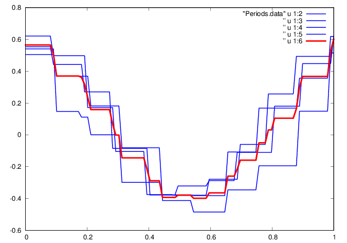
Extract the periods

octave>

nT = (shift(iPeak,-1)-iPeak+1)(1:nPeriods)

$(\begin{array}{cccc} 48 & 53 & 54 & 48 \end{array})$

octave>

nTmax = max(nT);

tT = zeros([nTmax,nPeriods]);

aT = zeros([nTmax,nPeriods]);

TT = zeros([nPeriods,1]);

i=1; while(i<=nPeriods)

tT(1:nT(i),i) = tGi(iPeak(i):iPeak(i+1));

aT(1:nT(i),i) = aGi(iPeak(i):iPeak(i+1));

TT(i) = tT(nT(i),i) - tT(1,i);

i++;

endwhile;

disp(TT');

0.53811 0.59536 0.60681 0.53811

octave>

i=1; while(i<=nPeriods)

tT(1:nT(i),i) = tT(1:nT(i),i) - tT(1,i);

tT(1:nT(i),i) = tT(1:nT(i),i)/TT(i);

amp = max(aT(1:nT(i),i)) - min(aT(1:nT(i),i));

aT(1:nT(i),i) = aT(1:nT(i),i)/amp;

i++;

endwhile;

octave>

nTi=100;

dt=1./(nTi-1); ti=(0:nTi-1)*dt; ti=ti';

aTi=zeros([nTi,nPeriods]); g=zeros([nTi,1]);

i=1; while(i<=nPeriods)

ai = interp1(tT(1:nT(i),i),aT(1:nT(i),i),ti',"nearest");

aTi(:,i) = ai;

g = g + ai';

i++;

endwhile;

g = g/nPeriods;

g = g/(max(g)-min(g));

octave>

fid=fopen('Periods.data','w');

ta = [ti aTi g];

fprintf(fid,'%f %f %f %f %f %f\n',ta');

fclose(fid);

fid=fopen(strcat(strcat('AveragePeriod.',LastName),'.data'),'w');

ta = [ti g];

fprintf(fid,'%f %f \n',ta');

fclose(fid);

octave>

GNUplot]

cd '/home/student/courses/MATH590/NUMdata'

set terminal postscript eps enhanced color

set style line 1 lt 2 lc rgb "red" lw 6

set style line 2 lt 2 lc rgb "green" lw 3

set style line 3 lt 2 lc rgb "blue" lw 3

plot "Periods.data" u 1:2 w l ls 3, ” u 1:3 w l ls 3, ” u 1:4 w l ls 3, ” u 1:5 w l ls 3, ” u 1:6 w l ls 1

GNUplot]

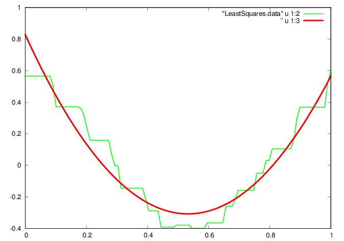
Question 5. What are the potential drawbacks of defining an “average” gait? Consider the limiting cases of too few or very many sample periods.

2.4Least squares

Seek a more economical representation of the average gait waveform, currently stored as a vector $𝐠 \in ℝ^{m}$ of the vertical acceleration values at times within the vector $𝐭 \in ℝ^{m}$ . For example, consider approximating the waveform by a parabola $p (t) = c_{0} + c_{1} t + c_{2} t^{2}$ , leading to the least squares problem

{min}_{𝐜 \in ℝ^{3}} || 𝐋 𝐜 - 𝐠 ||, 𝐋 = (\begin{array}{lll} 𝟏 & 𝐭 & 𝐭^{2} \end{array}) \in ℝ^{m \times 3}, 𝐭^{k} = {(\begin{array}{lll} t_{1}^{k} & \dots & t_{m}^{k} \end{array})}^{T} .

(1)

A solution is found by projection onto the column space of $𝐋$ ,

𝐐 𝐑 = 𝐋, 𝐏_{C (𝐋)} = 𝐐 𝐐^{T}, 𝐏_{C (𝐋)} 𝐠 = 𝐐 𝐑 𝐜 \Rightarrow 𝐑 𝐜 = 𝐐^{T} 𝐠 .

(2)

octave>

L=[ti.^0 ti ti.^2]; [Q,R]=qr(L,0); [size(Q); size(R)]

$(\begin{array}{cc} 100 & 3 \\ 3 & 3 \end{array})$

octave>

c = R \ Q'*g

$(\begin{array}{c} 0.82834 \\ - 4.2652 \\ 4.003 \end{array})$

octave>

p = L*c;

fid=fopen('LeastSquares.data','w');

ta = [ti g p];

fprintf(fid,'%f %f %f\n',ta');

fclose(fid);

octave>

GNUplot]

cd '/home/student/courses/MATH590/NUMdata'

set terminal postscript eps enhanced color

set style line 1 lt 2 lc rgb "red" lw 6

set style line 2 lt 2 lc rgb "green" lw 3

set style line 3 lt 2 lc rgb "blue" lw 3

plot "LeastSquares.data" u 1:2 w l ls 2, ” u 1:3 w l ls 1

GNUplot]

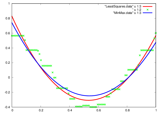
Question 6. What gait information is lost in the least squares approximation?

2.5Min-max

An alternative representation is through a linear combination of Chebyshev polynomials,

q (t) = d_{0} T_{0} (t) + d_{1} T_{1} (t) + d_{2} T_{2} (t)

known to be a good approximation of the min-max polynomial of the data. The coefficient vector $𝐝 \in ℝ^{3}$ is more difficult to find by comparison to the least squares case, and is carried out through a procedure known as the exchange algorithm, implemented in Octave by the polyfitinf function.

octave>

d=polyfitinf(2,nTi,0,ti,g,5.0E-7,nTi)

$(\begin{array}{ccc} 3.3996 & - 3.665 & 0.74003 \end{array})$

octave>

q = polyval(d,ti);

fid=fopen('MinMax.data','w');

ta = [ti g q];

fprintf(fid,'%f %f %f\n',ta');

fclose(fid);

octave>

GNUplot]

cd '/home/student/courses/MATH590/NUMdata'

set terminal postscript eps enhanced color

set style line 1 lt 2 lc rgb "red" lw 6

set style line 2 lt 2 lc rgb "green" lw 3

set style line 3 lt 2 lc rgb "blue" lw 6

plot "LeastSquares.data" u 1:3 w l ls 1, ” u 1:2 w p ls 2, "MinMax.data" u 1:3 w l ls 3

GNUplot]

Question 7. Which gait approximation is better suited to walker identification, least squares or min-max? Explain your reasoning.

Save the coefficients of the two representations (least-squares and Chebyshev)

octave>

fid=fopen(strcat(strcat('PolyCoef.',LastName),'.data'),'w');

ta = [c d'];

fprintf(fid,'%f %f\n',ta');

fclose(fid);

octave>