MATH661

1.Rate and order of convergence

Exercise 1. Estimate the rate and order of convergence of a sequence from the samples

1, \frac{0.9}{2}, \frac{0.81}{4}, \frac{0.729}{8} .

Exercise 2. Construct a convergence plot for the sequence

a_{n} = \frac{1}{\ln n} .

Can you estimate the rate and order of convergence?

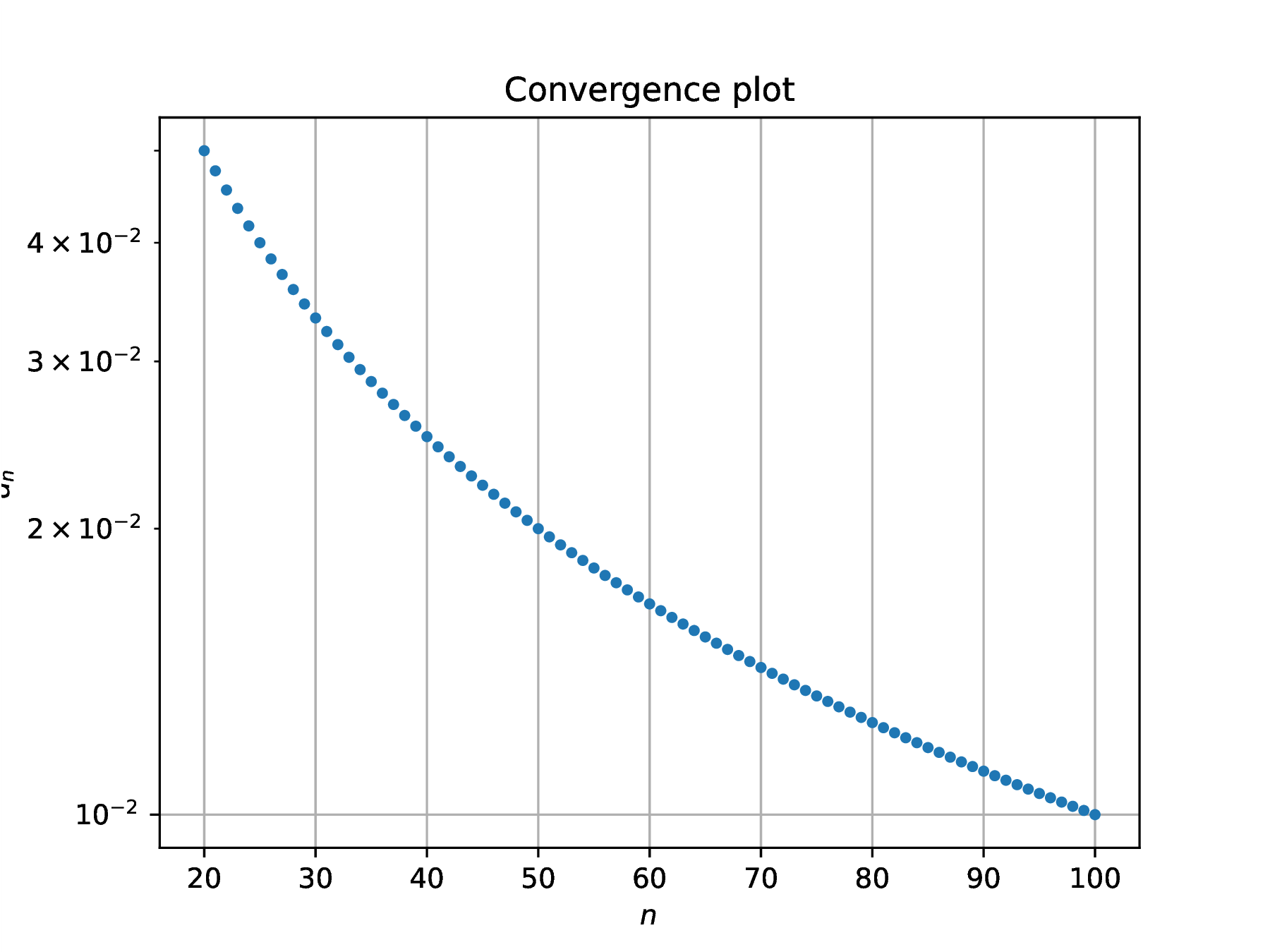
Solution. Since ${lim}_{n \to \infty} a_{n} = a = 0$ , note that the distance to the limit $d_{n} = | a_{n} - a |$ is simply $d_{n} = a_{n}$ for $n > 1$ . For large $n$ , the convergence behavior is given by $d_{n + 1} = s d_{n}^{q}$ , leading to $\lg (d_{n + 1}) = q \lg (d_{n}) + \lg (s)$ upon taking decimal logarithms. In practical computation, $n$ is chosen between some upper bound $N$ dictated by allowed computational effort and a lower bound $M$ needed to start observing convergence

M ⩽ n ⩽ N .

The computed terms ${d_{n}}$ allow estimation of $(s, q)$ by linear regression (least squares fitting) expressed as

[\begin{array}{ll} 1 & \lg (d_{M}) \\ 1 & \lg (d_{M + 1}) \\ ⋮ & ⋮ \\ 1 & \lg (d_{N - 1}) \end{array}] [\begin{array}{l} \lg (s) \\ q \end{array}] ≅ [\begin{array}{l} \lg (d_{M + 1}) \\ \lg (d_{M + 2}) \\ ⋮ \\ \lg (d_{N}) \end{array}] \Leftrightarrow 𝑨 𝒙 ≅ 𝒚 .

The Julia instruction $x = A \ y$ carries out the linear regression (also a feature of Matlab/Octave).

∴	M=20; N=100; n=M:N; a=1 ./ log.(n); d=a; lgd=log10.(d);

∴	m=N-M; y=lgd[2:m+1]; A=ones(m,2); A[:,2]=lgd[1:m];

∴	x=A\y; s=10^x[1]; q=x[2]; [s q]

$[\begin{array}{cc} 0.9560115307957512 & 0.9712804466056952 \end{array}]$ (1)

∴

From the above, obtain order of convergence $q ≅ 0.97$ (sublinear convergence), and rate of convergence $s ≅ 0.96$ . The convergence plot highlights this sublinear convergence behavior.

∴	x=n; y=d; clf(); semilogy(x,y,"."); grid("on");

∴	xlabel(L"$n$"); ylabel(L"$d_n$"); title("Convergence plot");

∴	savefig(homedir()*"/courses/MATH661/images/E02Fig01.eps");

∴

Figure 1. Sub-linear convergence behavior of the sequence $a_{n} = 1 / \log (n)$ .

Exercise 3. Construct a convergence plot for the sequence

a_{n} = e^{- n} .

Can you estimate the rate and order of convergence?

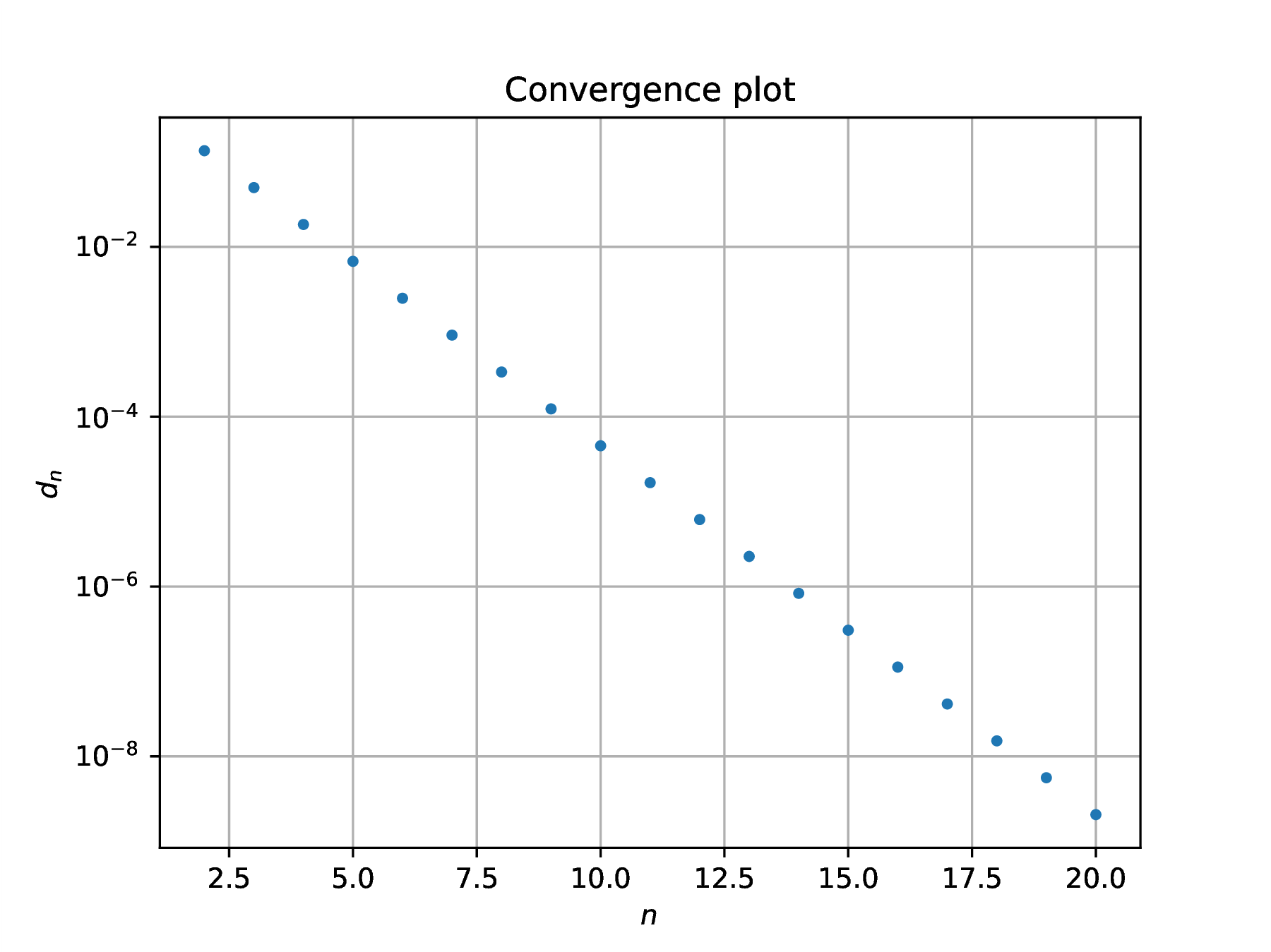
Solution. Again, ${lim}_{n \to \infty} a_{n} = 0$ , hence $d_{n} = a_{n}$ for $n ⩾ 1$ . Repeat the above computation for the new sequence choosing lower values for $M, N$ since $e^{- n}$ is expected to converge to zero faster than $1 / \ln n$ .

∴	M=2; N=20; n=M:N; a=exp.(-n); d=a; lgd=log10.(d);

∴	m=N-M; y=lgd[2:m+1]; A=ones(m,2); A[:,2]=lgd[1:m];

∴	x=A\y; s=10^x[1]; q=x[2]; [s q]

$[\begin{array}{cc} 0.36787944117144333 & 0.9999999999999999 \end{array}]$ (2)

Linear convergence is obtained, $q = 1$ , and the rate of convergence $s ≅ 0.37$ . The order of convergence is only slightly better than the previous sequence and faster convergence arise from the marked difference in rate of convergence.

∴	x=n; y=d; clf(); semilogy(x,y,"."); grid("on");

∴	xlabel(L"$n$"); ylabel(L"$d_n$"); title("Convergence plot");

∴	savefig(homedir()*"/courses/MATH661/images/E02Fig02.eps");

∴

Figure 2. Sub-linear convergence behavior of the sequence $a_{n} = e^{- n}$ .

Exercise 4. Plot in logarithmic coordinates $a_{n} = \sqrt{n}$ , $a_{n + 1} - a_{n}$ , $a_{n + 2} - a_{n}$ , $\dots$ , $a_{n + 10} - a_{n}$ . Do the $a_{n + k} - a_{n}$ sequences converge?

BoundsError([0.05, 0.047619047619047616, 0.045454545454545456, 0.043478260869565216, 0.041666666666666664, 0.04, 0.038461538461538464, 0.037037037037037035, 0.03571428571428571, 0.034482758620689655, 0.03333333333333333, 0.03225806451612903, 0.03125, 0.030303030303030304, 0.029411764705882353, 0.02857142857142857, 0.027777777777777776, 0.02702702702702703, 0.02631578947368421, 0.02564102564102564, 0.025, 0.024390243902439025, 0.023809523809523808, 0.023255813953488372, 0.022727272727272728, 0.022222222222222223, 0.021739130434782608, 0.02127659574468085, 0.020833333333333332, 0.02040816326530612, 0.02, 0.0196078431372549, 0.019230769230769232, 0.018867924528301886, 0.018518518518518517, 0.01818181818181818, 0.017857142857142856, 0.017543859649122806, 0.017241379310344827, 0.01694915254237288, 0.016666666666666666, 0.01639344262295082, 0.016129032258064516, 0.015873015873015872, 0.015625, 0.015384615384615385, 0.015151515151515152, 0.014925373134328358, 0.014705882352941176, 0.014492753623188406, 0.014285714285714285, 0.014084507042253521, 0.013888888888888888, 0.0136986301369863, 0.013513513513513514, 0.013333333333333334, 0.013157894736842105, 0.012987012987012988, 0.01282051282051282, 0.012658227848101266, 0.0125, 0.012345679012345678, 0.012195121951219513, 0.012048192771084338, 0.011904761904761904, 0.011764705882352941, 0.011627906976744186, 0.011494252873563218, 0.011363636363636364, 0.011235955056179775, 0.011111111111111112, 0.01098901098901099, 0.010869565217391304, 0.010752688172043012, 0.010638297872340425, 0.010526315789473684, 0.010416666666666666, 0.010309278350515464, 0.01020408163265306, 0.010101010101010102, 0.01], (21:99,))

Approximation Techniques - Exercises

1.Rate and order of convergence

2.Aitken acceleration

3.Approximation techniques