Solve the problems for your appropriate course track. Problems probe understanding of the course concepts. Formulate your answers clearly and cogently. Sketch out an approach on scratch paper first. Then briefly transcribe the approach to the answer you turn in, followed by appropriate calculations and conclusions, within allotted time. Use concise, complete English sentences in the description of your approach.

Each question is meant to be completely answered and transcribed from proof to final copy within thirty minutes. Concentrate foremost on clear exposition of the concept underlying your approach.

1Track 1

1. Consider the ballistic missile trajectory problem of national defense interest. From measurements of the positions $x_i=x\left(t_i\right)$ at successive times $t_i$, $i=0,...,n$ predict the target reached at time $T>t_n$. Formulate a procedure to predict $x\left(T\right)$, assuming the missile is known to follow a parabolic trajectory.

   Solution. The parabolic trajectory is expressed through a quadratic approximant

   ${\displaystyle x\left(t\right)=c_0+c_{1}t+c_2{t}^2.}$

   The coefficients $a,b,c$ are the solution of the least squares problem

   ${\displaystyle {min}_{𝒄}{||𝑨𝒄-𝒙||}_2,}$

   with

   ${\displaystyle {𝒕}^j=\left[\begin{array}{l}{t}_0^j\\ t_1^j\\ ⋮\\ t_n^j\end{array}\right],𝑨=\left[\begin{array}{lll}{𝒕}^0& {𝒕}^1& {𝒕}^2\end{array}\right],𝒄=\left[\begin{array}{l}{c}_0\\ c_1\\ c_2\end{array}\right],𝒙=\left[\begin{array}{l}{x}_0\\ x_1\\ ⋮\\ x_n\end{array}\right].}$

   To solve the least squares problem:

   • Compute $QR$-factorization, $𝑸𝑹=𝑨$

   • Solve $𝑹𝒄={𝑸}^T𝒙$.

2. Construct a quadrature formula for integrals of the form

   ${\displaystyle \underset{0}{\overset{\infty }{\int }}{e}^{-\alpha t}f\left(t\right)dt.}$

   Solution. Assuming sampling data $𝒟=\{(t_i,f_i=f\left(t_i\right)),i=0,1,..,n\}$, find the weights $w_i$ of the quadrature

   ${\displaystyle \underset{0}{\overset{\infty }{\int }}{e}^{-\alpha t}f\left(t\right)dt\cong \sum _{i=0}^n{w}_i{f}_i}$

   by imposing the moment conditions

   ${\displaystyle \underset{0}{\overset{\infty }{\int }}{e}^{-\alpha t}{t}^{j}dt=\sum _{i=0}^n{w}_i{t}_i^j,k=0,1,..,n}$

   a linear system with a Vandermonde system matrix

   ${\displaystyle 𝑽𝒘=𝒃.}$

   The moments are analytically evaluated through integration by parts

   ${\displaystyle b_j=\underset{0}{\overset{\infty }{\int }}{e}^{-\alpha t}{t}^{j}dt=\frac{j}{\alpha }\underset{0}{\overset{\infty }{\int }}{e}^{-\alpha t}{t}^{j}dt=\frac{j}{\alpha }{b}_{j-1}=\frac{j!}{a^{j+1}},b_0=\frac{1}{\alpha }.}$

3. Find the best approximant in the least squares sense of $\sin t$ within $\mathrm{span}\{1,t,t^2\}$.

   Solution. Orthonormalize $\{1,t,t^2\}$ using Gram-Schmidt in a Hilbert space with scalar product

   ${\displaystyle (f,g)=\underset{-\pi }{\overset{\mathrm{\pi }}{\int }}f\left(t\right)g\left(t\right)dt.}$

   Obtain the orthonormal set $\{p_0\left(t\right),p_1\left(t\right),p_2\left(t\right)\}$. The least squares approximant $g$ is

   ${\displaystyle g\left(t\right)=(\sin ,p_0)p_0\left(t\right)+(\sin ,p_1)p_1\left(t\right)+(\sin ,p_2)p_2\left(t\right).}$

   Gram-Schmidt calculations:

   ${\displaystyle p_0\left(t\right)=\frac{1}{(1,1)}=\frac{1}{\sqrt{2\pi }}.}$ ${\displaystyle q_1\left(t\right)=t-(t,p_0)p_0=t}$ ${\displaystyle p_1\left(t\right)=\frac{q_1\left(t\right)}{(q_1,q_1)}=\sqrt{\frac{3}{2{\pi }^3}}t}$ ${\displaystyle q_2\left(t\right)=t^2-(t^2,p_1)p_1\left(t\right)-(t^2,p_0)p_0\left(t\right)=t^2-\frac{{\pi }^2}{3}}$ ${\displaystyle p_2\left(t\right)=\frac{q_2\left(t\right)}{(q_2,q_2)}=\sqrt{\frac{45}{8{\pi }^5}}(t^2-\frac{{\pi }^2}{3}).}$

   Coefficient of $\sin t$ on orthonormal basis (use fact that sin is odd, $p_0,p_2$ are even)

   ${\displaystyle (\sin ,p_0)=0,(\sin ,p_2)=0}$ ${\displaystyle (\sin ,p_1)=\sqrt{\frac{6}{\pi }}.}$

   The best approximant is

   ${\displaystyle \sin t\cong \sqrt{\frac{6}{\pi }}\sqrt{\frac{3}{2{\pi }^3}}t=\frac{3}{{\pi }^2}t.}$

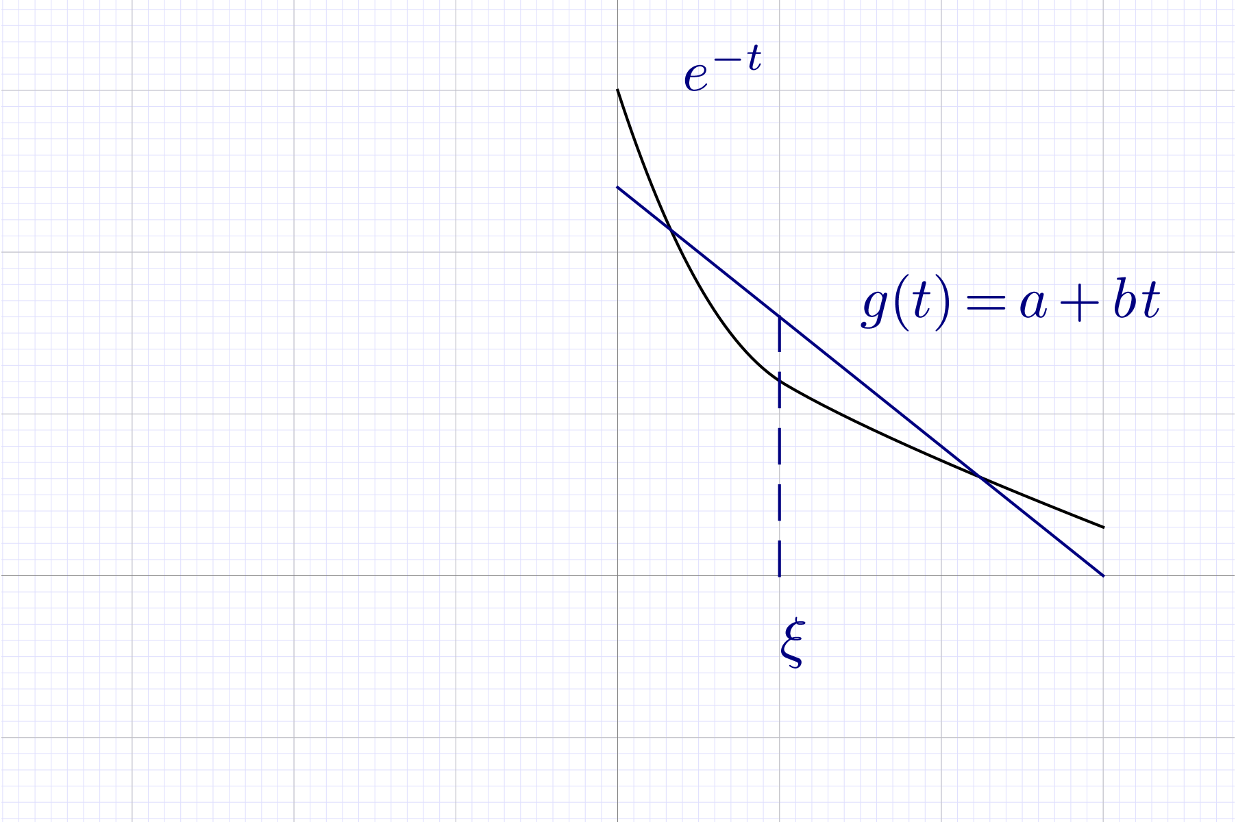
4. Find the best inf-norm approximant of $f:[0,1]\to ℝ$, $f\left(t\right)=e^{-t}$ by a first-degree polynomial.

   By equioscillation theorem $g\left(t\right)=a+bt$ satisfies the alternating difference conditions

   ${\displaystyle e^0-g\left(0\right)=\delta ,g\left(\xi \right)-e^{-\xi }=\delta ,e^{-1}-g\left(1\right)=\delta ,}$

   and the stationarity condition

   ${\displaystyle {\left[\frac{d}{dt}(g\left(t\right)-e^{-t})\right]}_{t=\xi }=0.}$

   These lead to the system

   ${\displaystyle 1-a=\delta ,a+b\xi -e^{-\xi }=\delta ,e^{-1}-(a+b)=\delta ,b+e^{-\xi }=0.}$

   Eliminaing $\delta ,\xi$ leads to a system for $a,b$ with solution

   ${\displaystyle b=\frac{1-e}{e},\xi =1-\ln (e-1),a=\frac{1}{2}[1+e^{-\xi }-\xi \frac{1-e}{e}],}$

   defining the best inf-norm linear approximant of $e^{-t}$

   Figure 1.

5. Propose a scheme to solve the integro-differential equation

   ${\displaystyle \frac{dy}{dt}+y=\underset{0}{\overset{t}{\int }}\sin (t-\tau )y\left(\tau \right)d\tau ,}$

   for $y:ℝ\to ℝ$. Apply all relevant course concepts to analyze the scheme.

   Solution. Consider an equidistant sampling at $t_i=ih$, $y_i\cong y\left(t_i\right)$, and discretize the derivative through forward differencing (forward Euler, second-order one-step error)

   ${\displaystyle y_{i+1}-y_i=-h{y}_i+\sum _{j=1}^{i+1}\underset{t_{j-1}}{\overset{t_j}{\int }}\sin (t-\tau )y\left(\tau \right)d\tau .}$

   Over $[t_{j-1},t_j]$ approximate the integrand the scond-order accurate trapezoid rule (to maintain Euler one-step error)

   ${\displaystyle y_{i+1}-y_i=-h{y}_i+\frac{h}{2}\sum _{j=1}^{i+1}[\sin (t_i-t_{j-1})y_{j-1}+\sin (t_i-t_j)y_j]\Rightarrow }$ ${\displaystyle y_{i+1}-y_i=-h{y}_i+\frac{h}{2}[\sum _{j=0}^i\sin (t_{i+1}-t_j)y_j+\sum _{j=1}^{i+1}\sin (t_i-t_j)y_j]\Rightarrow }$ ${\displaystyle y_{i+1}-y_i=-h{y}_i+\frac{h}{2}\sin \left(t_{i+1}\right)y_0+\frac{h}{2}\sum _{j=1}^i[\sin (t_{i+1}-t_j)+\sin (t_i-t_j)]y_j+\frac{h}{2}\sin (t_i-t_{i+1})y_{i+1}\Rightarrow }$ ${\displaystyle (1+\frac{h\sin h}{2})y_{i+1}=(1+h)y_i++\frac{h}{2}\sin \left(t_{i+1}\right)y_0+h\cos h\sum _{j=1}^i\sin [2(i-j)h+1]y_j.}$

   The above scheme has one step error of $𝒪\left(h^2\right)$, overall error of $𝒪\left(h\right).$

2Track 2

1. Construct an approximant of $e^{𝑨\left(t\right)}$ where $𝑨\left(t\right)\in {ℝ}^{m\times m}$ is a symmetric positive definite matrix-valued function of $t\in ℝ$.

   Solution. Many approaches are possible; the question tests understanding of the overall course material to the level of proposing a viable technique.

   Simplest approach. $𝑨\left(t\right)$ s.p.d. implies it is unitarily diagonalizable, i.e., $\forall t$, $\exists 𝑸\left(t\right)\in {ℝ}^{m\times m}$, $𝑸{𝑸}^T={𝑸}^T𝑸=𝑰$ such that

   ${\displaystyle 𝑨\left(t\right)=𝑸\left(t\right)𝚲\left(t\right){𝑸}^T\left(t\right).}$

   By definition

   ${\displaystyle e^{𝑨\left(t\right)}=𝑰+\frac{1}{1!}𝑨\left(t\right)+\frac{1}{2!}{𝑨}^2\left(t\right)+\cdots =𝑸\left(t\right)[𝑰+\frac{1}{1!}𝚲\left(t\right)+\frac{1}{2!}{𝚲}^2\left(t\right)+\cdots ]{𝑸}^T\left(t\right)=𝑸\left(t\right)e^{𝚲\left(t\right)}{𝑸}^T\left(t\right).}$

   Introduce a piecewise constant approximation of $𝑨\left(t\right)\cong {𝑨}_k$ for $t\in [t_{k-1},t_k)$ (0-degree $B$-spline basis). Then

   ${\displaystyle e^{𝑨\left(t\right)}={𝑸}_k{e}^{{𝚲}_k}{𝑸}_k^T={𝑸}_k\mathrm{diag}({\lambda }_1^k,..,{\lambda }_m^k){𝑸}_k^T.}$

   Extension to a piecewise linear approximation

   ${\displaystyle 𝑨\left(t\right)={𝑨}_{k-1}+\left(\frac{t-t_{k-1}}{t_k-t_{k-1}}\right)({𝑨}_k-{𝑨}_{k-1})}$

   is not immediate since ${𝑨}_k-{𝑨}_{k-1}$ is not guaranteed to be s.p.d.

   Differential system approach. Recall that $y^{\text{'}}=ay$ has solution $y\left(t\right)=e^{at}{y}_0$, and $y^{\text{'}}=a\left(t\right)y$ has solution

   ${\displaystyle y\left(t\right)=\exp [\underset{0}{\overset{t}{\int }}a\left(\tau \right)d\tau ]y_0.}$

   With $𝑩\left(t\right)={𝑨}^{\text{'}}\left(t\right)$, ODE system

   ${\displaystyle {𝒚}^{\text{'}}=𝑩𝒚}$

   (1)

   has solution

   ${\displaystyle 𝒚\left(t\right)=\exp [\underset{0}{\overset{t}{\int }}𝑩\left(\tau \right)d\tau ]{𝒚}_0=\exp [\underset{0}{\overset{t}{\int }}{𝑨}^{\text{'}}\left(t\right)d\tau ]{𝒚}_0=\exp [𝑨\left(t\right)-𝑨\left(0\right)]{𝒚}_0=e^{𝑨\left(t\right)}{𝒚}_0-e^{{𝑨}_0}{𝒚}_0.}$

   Column $j$ of $e^{𝑨\left(t\right)}$ is obtained as

   ${\displaystyle e^{𝑨\left(t\right)}{𝒆}_j,}$

   i.e., the action of $e^{𝑨\left(t\right)}$ on the $j^{\mathrm{th}}$ column vector of the identity matrix. This can be obtained by any numerical scheme to solve the ODE system (1) starting from initial condition ${𝒚}_0={𝒆}_j$, amd adding $e^{{𝑨}_0}{𝒚}_0$ to the result.

2. Construct a quadrature formula for integrals of the form

   ${\displaystyle \underset{0}{\overset{\infty }{\int }}{e}^{𝑨\left(t\right)}𝒇\left(t\right)dt,}$

   where $$$𝑨\left(t\right)\in {ℝ}^{m\times m}$ is a symmetric negative definite matrix-valued function of $t\in ℝ$, and $𝒇:ℝ\to {ℝ}^m$ has Riemann integrable components.

   Solution. $𝑨\left(t\right)$ admits an orthogonal diagonalization

   ${\displaystyle 𝑨\left(t\right)=𝑸\left(t\right)𝚲\left(t\right){𝑸}^T\left(t\right)}$

   with $𝚲\left(t\right)=\mathrm{diag}({\lambda }_1,..,{\lambda }_m)$, ${\lambda }_i<0$, and the matrix exponential is

   ${\displaystyle e^{𝑨\left(t\right)}=𝑸\left(t\right){𝒆}^{𝚲\left(t\right)}{𝑸}^T\left(t\right).}$

   Define the scalar product

   ${\displaystyle {(𝒇,𝒈)}_{𝑨}=\underset{0}{\overset{\infty }{\int }}{𝒈}^T\left(t\right)e^{𝑨\left(t\right)}𝒇\left(t\right)dt=\underset{0}{\overset{\infty }{\int }}{𝒈}^T\left(t\right)𝑸\left(t\right){𝒆}^{𝚲\left(t\right)}{𝑸}^T\left(t\right)𝒇\left(t\right)dt.}$

   Approximate $𝒇\left(t\right),𝒈\left(t\right)$ on the $𝑸\left(t\right)$ basis

   ${\displaystyle 𝒇\left(t\right)\cong 𝑸\left(t\right)𝒄\left(t\right)\Rightarrow 𝒄\left(t\right)={𝑸}^T\left(t\right)𝒇\left(t\right),𝒈\left(t\right)\cong 𝑸\left(t\right)𝒅\left(t\right)\Rightarrow 𝒅\left(t\right)={𝑸}^T\left(t\right)𝒈\left(t\right),}$

   and obtain

   ${\displaystyle {(𝒇,𝒈)}_{𝑨}={(𝒄,𝒅)}_{𝚲}=\underset{0}{\overset{\infty }{\int }}{𝒅}^T\left(t\right){𝒆}^{𝚲\left(t\right)}𝒄\left(t\right)dt.}$

   Denote by ${\theta }_j$ the average value of ${\lambda }_j\left(t\right)$, $𝚯=\mathrm{diag}({\theta }_1,..,{\theta }_m)$ such that, by mean value theorem

   ${\displaystyle {(𝒇,𝒈)}_{𝑨}={(𝒄,𝒅)}_{𝚲}=\underset{0}{\overset{\infty }{\int }}{𝒅}^T\left(t\right){𝒆}^{𝚲\left(t\right)}𝒄\left(t\right)dt=\underset{0}{\overset{\infty }{\int }}{𝒅}^T\left(t\right){𝒆}^{𝚯}𝒄\left(t\right)dt.}$

   Interpret above as stating that standard Gauss-Laguerre quadrature formulas

   ${\displaystyle I\left(f\right)=\underset{0}{\overset{\infty }{\int }}{e}^{-t}f\left(t\right)dt\cong \sum _{i=0}^n{w}_i{f}_i=Q\left(f\right)}$

   are applicable to the individual components of

   ${\displaystyle 𝒄\left(t\right)={𝑸}^T\left(t\right)𝒇\left(t\right),}$

   using scale transformation

   ${\displaystyle \underset{0}{\overset{\infty }{\int }}{e}^{-\theta t}f\left(t\right)dt=\frac{1}{\theta }\underset{0}{\overset{\infty }{\int }}{e}^{-s}f(s/\theta )ds=\frac{1}{\theta }\underset{0}{\overset{\infty }{\int }}{e}^{-s}g\left(s\right)ds=\frac{1}{\theta }Q\left(g\right).}$

3. Find the best approximant of $𝒚\in {ℝ}^m$ within $C\left(𝑨\right)$, $𝑨\in {ℝ}^{m\times n}$ in a space with scalar product

   ${\displaystyle (𝒖,𝒗)={𝒖}^T𝑷𝒗,}$

   and norm

   ${\displaystyle ||𝒖||={(𝒖,𝒖)}^{1/2},}$

   where $𝑷\in {ℝ}^{m\times m}$ is symmetric positive definite. Verify the correspondence principle that for $𝑷=𝑰$ standard least-squares projection is obtained.

   Solution. Construct an orthogonal factorization $𝑨=𝑸𝑹$ using Gram-Schmidt and the specified scalar product

   Algorithm 1

   for $i=1:n$

   ${𝒒}_i={𝒂}_i$

   for $j=1:i-1$

   $r_{ji}={𝒒}_j^T𝑷{𝒒}_i$

   ${𝒒}_i={𝒒}_i-r_{ji}{𝒒}_j$

   end

   $r_{ii}={𝒒}_i^T𝑷{𝒒}_i$

   ${𝒒}_i={𝒒}_i/r_{\mathrm{ii}}$

   end

   The matrix $𝑸=\left[\begin{array}{lll}{𝒒}_1& & {𝒒}_n\end{array}\right]$ satisfies orthogonality relationship ${𝑸}^T𝑷𝑸=𝑰$

   ${\displaystyle \left[\begin{array}{l}{𝒒}_1^T\\ ⋮\\ {𝒒}_n^T\end{array}\right]𝑷\left[\begin{array}{lll}{𝒒}_1& ...& {𝒒}_n\end{array}\right]=\left[\begin{array}{l}{𝒒}_1^T\\ ⋮\\ {𝒒}_n^T\end{array}\right]\left[\begin{array}{lll}𝑷{𝒒}_1& ...& 𝑷{𝒒}_n\end{array}\right]=\left[\begin{array}{llll}{𝒒}_1^T𝑷{𝒒}_1& {𝒒}_1^T𝑷{𝒒}_2& ...& \\ & & & \\ & & & \end{array}\right]={𝑰}_n}$

   The residual $𝒓=𝒚-𝑨𝒙$ is orthogonal to $C\left(𝑨\right)$

   ${\displaystyle ({𝒒}_j,𝒚-𝑨𝒙)=0\Rightarrow {𝑸}^T𝑷(𝒕-𝑨𝒙)=0\Rightarrow {𝑸}^T𝑷𝑨𝒙={𝑸}^T𝑷𝒚\Rightarrow }$ ${\displaystyle {𝑸}^T𝑷𝑸𝑹𝒙={𝑸}^T𝑷𝒚\Rightarrow 𝑹𝒙={𝑸}^T𝑷𝒚.}$

   The best approximant is $𝒛=𝑨𝒙=𝑸𝑹𝒙=𝑸{𝑸}^T𝑷𝒚$. For $𝑷=𝑰$, the Euclidean projection $𝒛=𝑸{𝑸}^T𝒚$

   is obtained.

4. Find the best inf-norm approximant of $f:[0,\infty )\to ℝ$, $f\left(t\right)=e^{-t}\cos t$ by a first-degree polynomial.

   Solution. The approximation error is

   ${\displaystyle \epsilon \left(t\right)=e^{-t}\cos t-(at+b)}$

   and the problem is stated as

   ${\displaystyle {min}_{a,b}{||\epsilon ||}_{\infty }={min}_{a,b}{sup}_{t\in ℝ}\left|\epsilon \left(t\right)\right|.}$

   Since $a\ne 0$ leads to infinitely large error, simplify the problem to

   ${\displaystyle {min}_b{sup}_{t\in ℝ}|e^{-t}\cos t-b|.}$

   The derivative

   ${\displaystyle f^{\text{'}}\left(t\right)=e^{-t}(-\sin t-\cos t)=-\sqrt{2}{e}^{-t}\sin (t+\frac{\pi }{4})}$

   has a root at $\xi =3\pi /4$ at which point

   ${\displaystyle f(3\pi /4)=-e^{-3\pi /4}/\sqrt{2}.}$

   Equioscillation theorem is satisfied by

   ${\displaystyle b=\frac{1}{2}(1-e^{-3\pi /4}/\sqrt{2}).}$

5. Consider the half-derivative operator $H$ defined as

   ${\displaystyle H^{2}f=H(Hf)=Df}$

   where $D=d/dt$ is the derivative operator. Propose a numerical scheme to evaluate $Hf$ that can be used to solve fractional differential equations.

   Solution. The differentiation operator $D$ is approximated to order $k$ in terms of the backward finite difference operator $\nabla =E^0-E^{-1}=I-E^{-1}$ by

   ${\displaystyle H^2\cong D_k=\frac{1}{h}(\nabla +\frac{{\nabla }^2}{2}+\frac{{\nabla }^3}{3}+\cdots +\frac{{\nabla }^k}{k}),}$

   where $\left(E^{k}f\right)\left(x_0\right)=f(x_0+kh)$ is the argument translation operator.

   Consider $k=1$

   ${\displaystyle H\cong \frac{1}{\sqrt{h}}{\nabla }^{1/2}=\frac{1}{\sqrt{h}}{(I-E^{-1})}^{1/2},}$

   and apply the generalized binomial expansion

   ${\displaystyle {(a+b)}^r=\sum _{k=0}^{\infty }\left(\begin{array}{l}r\\ k\end{array}\right)a^{r-k}{b}^k,}$

   for $a=I$, $b=-E^{-1}$, $r=1/2$. Obtain

   ${\displaystyle \sqrt{h}H\cong \left(\begin{array}{l}r\\ 0\end{array}\right){(-E^{-1})}^0+\left(\begin{array}{l}r\\ 1\end{array}\right){(-E^{-1})}^1+\left(\begin{array}{l}r\\ 2\end{array}\right){(-E^{-1})}^2+\cdots \Rightarrow }$ ${\displaystyle \sqrt{h}H\cong I-\frac{1}{2}{E}^{-1}-\frac{1}{8}{E}^{-2}-\frac{1}{16}{E}^{-3}-\frac{5}{128}{E}^{-4}-\cdots .}$

   Apply the above to fractional equation $Hf=g$, and obtain the scheme

   ${\displaystyle f_i-\frac{1}{2}{f}_{i-1}-\frac{1}{8}{f}_{i-2}-\frac{1}{16}{f}_{i-3}-\frac{5}{128}{f}_{i-4}=\sqrt{h}{g}_i.}$