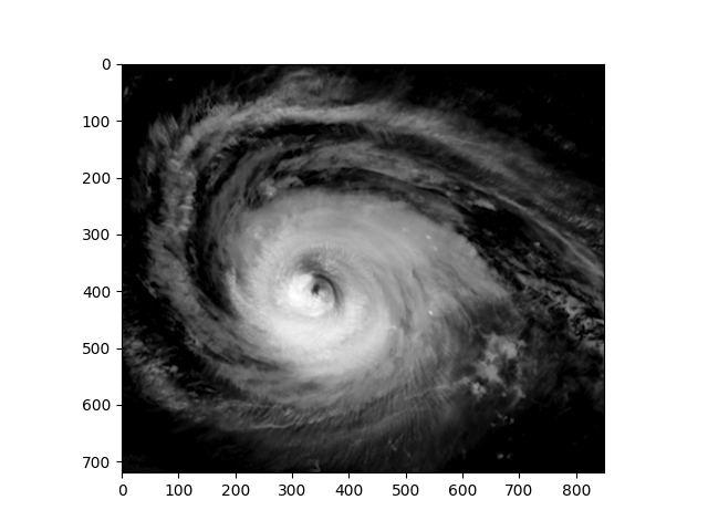
This homework marks your first foray into realistic scientific computation by applying concepts from linear algebra, specifically the singular value decomposition to the analysis of hurricane Lee, still active at this time.

1Image data

Processing of image data through the tools of linear algebra is often encountered, and in this assignment you shall work with satellite images of hurricane Lee of 2023 Season. Open the following folds and execute the code to set up your environment.

cd ~/courses/MATH661/data/weather

animate HurricaneLee.gif &

∴ 

import Pkg; Pkg.add("Images");

∴ 

Pkg.add(["FileIO","ImageIO"]);

∴ 

∴ 

using Images, FileIO, ImageIO

∴ 

∴ 

pre=homedir()*"/courses/MATH661/data/weather/";

∴ 

gif=load(pre*"HurricaneLee.gif");

∴ 

(mx,my,nf)=size(gif)

∴ 

∴ 

n=20; frame = Gray.(gif[:,:,n]);

∴ 

A = Float32.(frame); clf(); imshow(A,cmap="gray");

∴ 

hwdir=homedir()*"/courses/MATH661/homework/H03"; 

∴ 

savefig(hwdir*"/H03Fig01.png");

∴ 

Figure 1. Night-time satellite imagery of hurricane Lee. Superimposed on the familiar overall anti-cyclone pattern are small-scale features (lightning, cloud patterns in the arms). The SVD can be used to distinguish between small and large scale features.

2

1. Approximate $b\left(t\right)=t(\pi -t)(2\pi -t)$ on the interval $[0,2\pi )$ by the following series and study the convergence behavior of the solution. The pseudo-matrix $A\left(t\right)$ arising in the approximation is shown in each case

   1. Cosine series

      ${\displaystyle b\left(t\right)\cong \sum _{k=1}^n{y}_k\cos (kt),}$ ${\displaystyle A\left(t\right)=\left[\begin{array}{lllll}1& \cos \left(t\right)& \cos \left(2t\right)& \dots & \cos (nt)\end{array}\right],A:ℝ\to {ℝ}^{n+1}.}$

   2. Trigonometric series

      ${\displaystyle b\left(t\right)\cong \sum _{k=1}^n[x_k\cos (kt)+y_k\sin (kt)],}$ ${\displaystyle A\left(t\right)=\left[\begin{array}{llllllll}1& \cos \left(t\right)& \sin \left(t\right)& \cos \left(2t\right)& \sin \left(2t\right)& \dots & \cos (nt)& \sin (nt)\end{array}\right],A\left(t\right):ℝ\to {ℝ}^{2n+1}.}$

   3. Sine series

      ${\displaystyle b\left(t\right)\cong \sum _{k=1}^n{y}_k\sin (kt),}$ ${\displaystyle A\left(t\right)=\left[\begin{array}{llll}\sin \left(t\right)& \sin \left(2t\right)& \dots & \sin (nt)\end{array}\right],A:ℝ\to {ℝ}^n.}$

   4. Triangle wave series

      ${\displaystyle b\left(t\right)\cong \sum _{k=1}^n{z}_k{W}_k(t),}$ ${\displaystyle A\left(t\right)=\left[\begin{array}{llll}{W}_1\left(t\right)& W_2\left(t\right)& \dots & W_n(t)\end{array}\right],A:ℝ\to {ℝ}^n,}$

      with

      ${\displaystyle W_k\left(t\right)=1-4|\frac{1}{2}-⟦\frac{1}{4}+\frac{kt}{2\pi }⟧|,}$

      where $⟦x⟧$ is the fractional part of $x$, e.g., $⟦1.15⟧=0.15$.

2. Study the analytical theory underlying the above approximations by considering the following.

   1. State the convergence theorem for Fourier series and the Fourier coefficient formulas (see, e.g., [1]). Analytically compute the Fourier coefficients for $b\left(t\right)=t(\pi -t)(2\pi -t)$. Use of a symbolic computation package (e.g., Maxima, Mathematica) eliminates tedious hand computation.

   2. Compare the analytically computed Fourier coefficients with the numerical results obtained in Problem 1, a)-c). Assess the analytically predicted Fourier series convergence by comparison to the numerical results.

   3. Carry out series approximations as in Problem 1, a)-d) of

      ${\displaystyle c\left(t\right)=\frac{{\pi }^3}{4}[H\left(t\right)-2H(.t-\pi ).]}$

      where $H\left(x\right)$ is the Heaviside step function

      ${\displaystyle H\left(x\right)=\{\begin{array}{ll}0& x<0\\ 1& x>0\end{array}..}$

   4. Again, compare analytically evaluated Fourier coefficients with numerical results. How do the approximations of $c\left(t\right)$ behave differently from those of $b\left(t\right)$?

Bibliography