MATH661 HW03 - SVD applications

MATH661 HW03 - SVD applications

Posted: 09/13/23

Due: 09/20/23, 11:59PM

Tracks 1 & 2: 1. Track 2: 2.

This homework marks your first foray into realistic scientific computation by applying concepts from linear algebra, specifically using the singular value decomposition to analyze hurricane Lee, still active at this time.

1Problem setup

1.1Image data

Processing of image data through the tools of linear algebra is often encountered, and in this assignment you shall work with satellite images of hurricane Lee of 2023 Season. Open the following folds and execute the code to set up your environment.

$\circ$ The following commands within a BASH shell brings up an animation of hurricane Lee (ImageMagick package must be installed and in the system path.

$\circ$ The model will use various Julia packages to process image data, carry out linear algebra operations. The following commands build the appropriate Julia environment. The Julia packages are downloaded, compiled and stored in your local Julia library. Note: compiling the Images package takes a long time and it's best to do this within a terminal window. Compiling the packages need only be done once.

$\circ$ Once compiled, packages are imported into the current environment

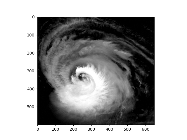
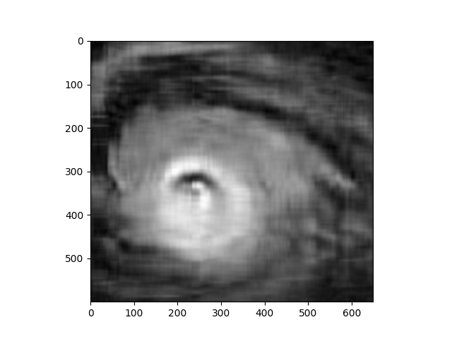
$\circ$ With appropriate packages in place and available, the satellite imagery can be imported into the Julia environment and used to insert images such as the one in Fig. (1).

∴	pre=homedir()*"/courses/MATH661/data/weather/";

∴	gif=load(pre*"HurricaneLee.gif");

∴	(mx,my,nf)=size(gif)

$[\begin{array}{c} 720 \\ 850 \\ 100 \end{array}]$ (1)

∴

The following commands display the $n^{th}$ frame in the animation, and save it within a homework directory. Use this template to save interesting images

∴	n=20; frame = Gray.(gif[:,:,n]);

∴	A = Float32.(frame); clf(); imshow(A,cmap="gray");

∴	hwdir=homedir()*"/courses/MATH661/homework/H03";

∴	savefig(hwdir*"/H03Fig01.png");

∴

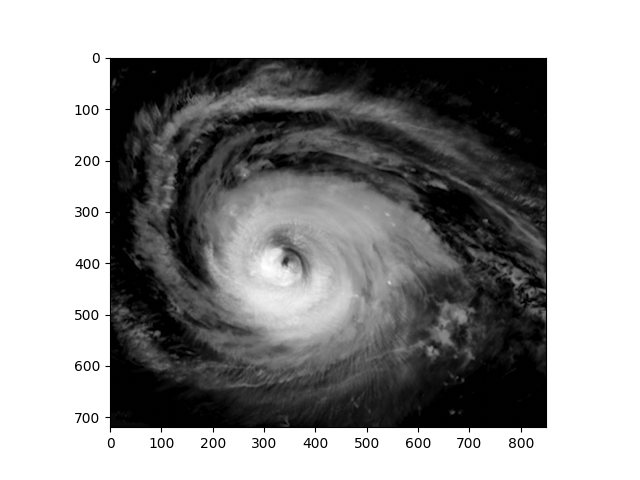
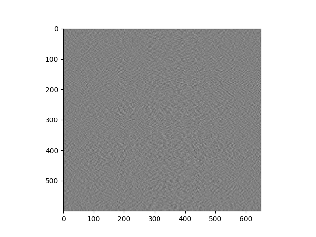
$\circ$ Image data must be quantified, i.e., transformed into numbers prior to analysis. In this case matrices of 32-bit floats are obtained from the gray-scale intensity values associated with each pixel. The 720 by 850 pixel images might be too large for machines with limited hardware resources, so adapt the window to obtain reasonable code execution times, Fig. 2.

∴	window = Gray.(gif[51:650,101:750,:]);

∴	data = Float32.(window); clf(); imshow(data[:,:,nf],cmap="gray");

∴	(nx,ny,nf) = size(data)

$[\begin{array}{c} 600 \\ 650 \\ 100 \end{array}]$ (2)

∴

Figure 1. Night-time satellite imagery of hurricane Lee. Superimposed on the familiar overall anti-cyclone pattern are small-scale features (lightning, cloud patterns in the arms). The SVD can be used to distinguish between small and large scale features.

Figure 2. Data window of a time snapshot of hurricane Lee.

1.2Computing the SVD

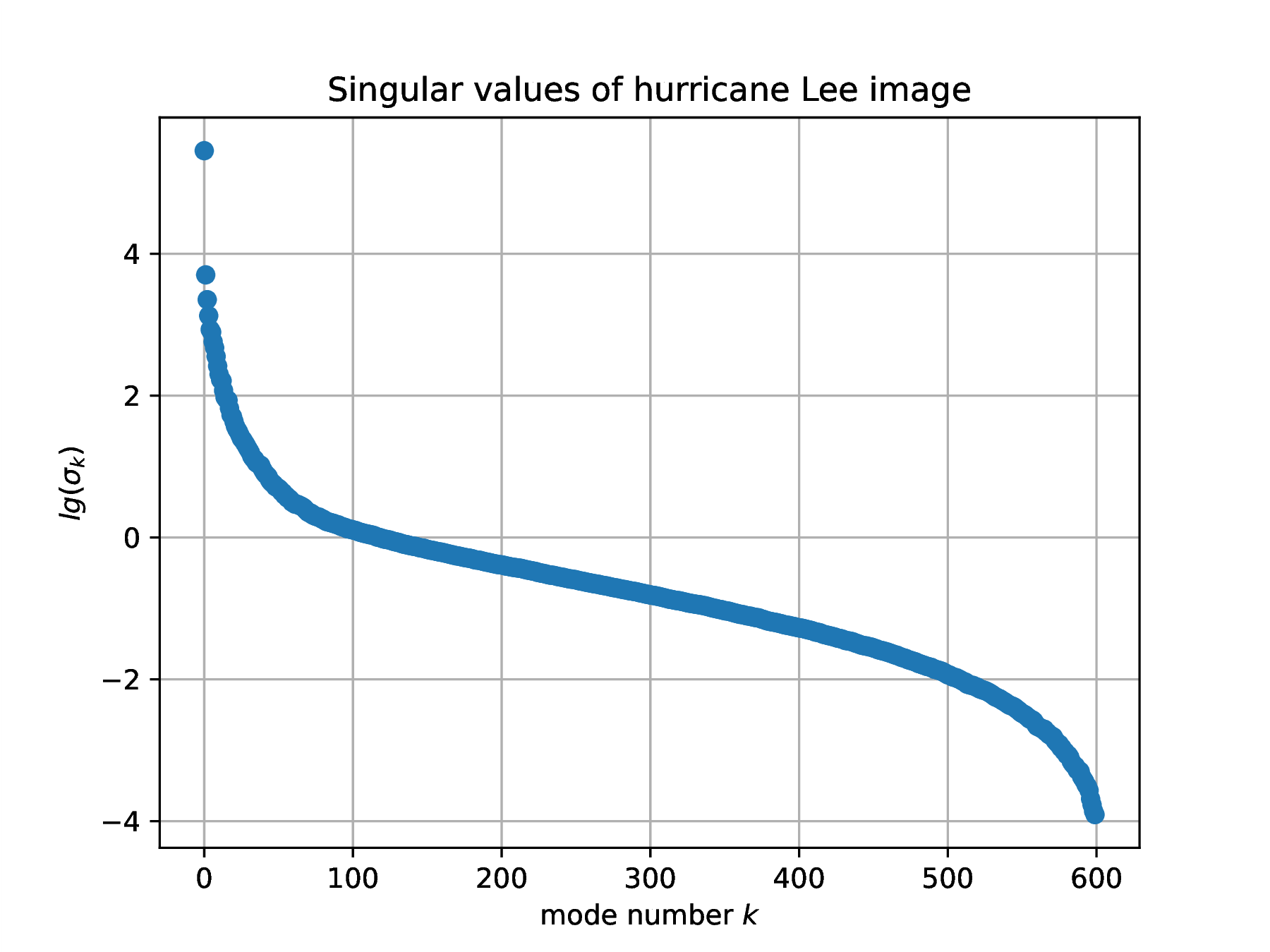
The SVD of the array of floats obtained from an image identifies correlations in gray-level intensity between pixel positions, an encoded description of weather physics. Here are the Julia instructions to compute the SVD of one frame of image data. It is instructive to plot the singular values $Σ = diag (σ_{1}, σ_{2}, \dots)$ , in log coordinates.

∴	n=32; A=data[:,:,n]; U,S,V=svd(A);

∴	clf(); plot(log.(S),"o"); xlabel(L"mode number $k$"); ylabel(L"lg(\sigma_k)");

∴	title("Singular values of hurricane Lee image"); grid("on");

∴	savefig(hwdir*"/H03Fig03a.eps");

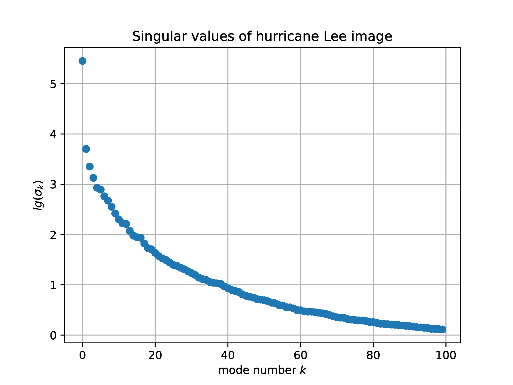
∴	clf(); plot(log.(S[1:100]),"o"); xlabel(L"mode number $k$"); ylabel(L"lg(\sigma_k)");

∴	title("Singular values of hurricane Lee image"); grid("on");

∴	savefig(hwdir*"/H03Fig03b.eps");

∴

Figure 3. The singular values of a hurricane satellite image rapidly decay from $\sim 10^{5}$ to $\sim 10^{0}$ , a five order-of-magnitude decrease over the first 100 modes (singular vectors). This indicates considerable data compression is possible.

$\circ$ Define a function rsvd to sum the rank-one updates from $p$ to $q$ from an SVD,

𝑨 = 𝑼 𝚺 𝑽^{T} ≅ 𝑩 = \sum_{k = p}^{q} σ_{j} 𝒖_{j} 𝒗_{j}^{T} .

The sum from $p = 1$ to $q$ contains the first $q$ dominant correlations, identified as large scale weather patterns. The sum from $p = 101$ to $q = 140$ can be identified as small scale patterns.

Figure 4. (Left) Reconstruction of hurricane Lee image from first $q = 12$ modes, showing large scale patterms. (Right) Correlated small-scale patterns obtained by sum of modes $p = 101$ to $q = 140$ .

2Common problems (both tracks)

Consider large-scale weather patterns $𝑩_{k}$ , $𝑩_{k - 1}$ , $𝑩_{k - 2}$ obtained from the $p$ most significant modes from frames $k, k - 1, k - 2$ (i.e., different times in the past). Assuming a constant rate of change leads to the prediction

$𝑷_{k} = 𝑩_{k - 1} + (𝑩_{k - 1} - 𝑩_{k - 2})$ (3)

for the known large-scale weather $𝑩_{k}$ . The prediction error is $ε_{k, 1} (p) = {|| 𝑷_{k} - 𝑩_{k} ||}_{F} / {|| 𝑩_{k} ||}_{F}$ . Present a plot of the prediction error for various values of $p$ over the recorded hurricane data. Analyze your results to answer the question: “can overall storm evolution be predicted by linear extrapolation of past data?”

Solution.
Repeat the above construction of an error plot for local weather patterns $𝑪_{k}, 𝑪_{k - 1}, 𝑪_{k - 2}$ for lesser significance modes from $p$ to $q$ , that lead to prediction
$𝑸_{k} = 𝑪_{k - 1} + (𝑪_{k - 1} - 𝑪_{k - 2}) .$
Analyze your results to answer the question: “are small-scale storm features predictable?”

Solution.
Repeat the above for combined large ( $𝑩$ ) and small scale ( $𝑪$ ) weather patterns. Experiment with different weights $u, v$ in the linear combination $u 𝑩 + v 𝑪$ , $u + v = 1$ .

Solution.
Formula (3) expresses a degree-one in time $t$ prediction
$𝑩 (t) = 𝑩_{k - 1} + (t - k + 1) (𝑩_{k - 1} - 𝑩_{k - 2}),$
evaluated at $t = k$ . Construct a quadratic prediction based upon data $𝑩_{k - 1}, 𝑩_{k - 2}, 𝑩_{k - 3}$ , and compare with degree-one prediction in question 1. Recall that a quadratic can be constructed from knowledge of three points. Again, experiment with various values of $k, p$ .

Solution.

3Track 2 questions

Use the SVD to investigate how familiar properties for $a \in ℝ$ might extend to matrices $𝑨 \in ℝ^{m \times m}$ . For example, on the real axis adding $- a$ to $a$ results in the null element, $a - a = 0$ , so we say $a$ is a distance $| a |$ from zero. This easily generalizes to $ℝ^{m}$ , and the minimal modification of $𝒂 \in ℝ^{m}$ to obtain zero is $- 𝒂$ , $𝒂 + (- 𝒂) = 𝟎$ , and $𝒂$ is distance $|| 𝒂 ||$ away from zero. Consider now matrices $𝑨 \in ℝ^{m \times m}$ , with $rank (𝑨) = m$ . How far is this matrix from “zero”? By “zero” we shall understand a singular matrix with $rank (𝑨) < m$ .

All real numbers $x \in ℝ$ can be obtained as the limit of a sequence of rationals ${p_{n} / q_{n}}$ , $p_{n}, q_{n} \in ℤ$ . We say that the rationals $ℚ$ is a dense subset of $ℝ$ . What about matrix spaces?

Find $𝑿$ of minimal norm such that $𝑨 + 𝑿$ is singular. State how far $𝑨$ is from “zero”?
Prove that any matrix in $ℝ^{m \times m}$ is the limit of a sequence of matrices of full rank, i.e., the set of full-rank matrices is a dense subset of $ℝ^{m \times m}$ .