MATH661

Lecture 2: Approximation techniques

1.Rate and order of convergence

The objective of scientific computation is to solve some problem $f (x) = 0$ by constructing a sequence of approximations ${x_{n}}_{n \in ℕ}$ . The condition suggested by mathematical analysis would be $x = {lim}_{n \to \infty} x_{n}$ , with $f (x) = 0$ . As already seen in the Leibniz series approximation of $π$ , acceptable accuracy might only be obtained for large $n$ . Since $f$ could be an arbitrarily complex mathematical object, such slowly converging approximating sequences are of little practical interest. Scientific computing seeks approximations of the solution with rapidly decreasing error. This change of viewpoint with respect to analysis is embodied in the concepts of rate and order of convergence.

Definition 1. ${x_{n}}_{n \in ℕ}$ converges to $x$ with rate $r \in (0, 1)$ and order $p$ if

${lim}_{n \to \infty} \frac{| x_{n + 1} - x |}{{| x_{n} - x |}^{p}} = r .$ (1)

As previously discussed, the above definition is of limited utility since:

The solution $x$ is unknown;

The limit $n \to \infty$ is impractical to attain.

Sequences converge faster for higher order $p$ or lower rate $r$ . A more useful approach is to determine estimates of the rate and order of convergence over some range of iterations that are sufficiently accurate. Rewriting (1) as

{lim}_{n \to \infty} (| x_{n + 1} - x | - r {| x_{n} - x |}^{p}) = 0,

suggests introducing the distance between successive iterates $d_{n} = | x_{n} - x_{n - 1} |$ , and considering the condition

| d_{n + 1} - s d_{n}^{q} | small for large n .

Definition 2. ${x_{n}}_{n \in ℕ}$ approximates $x$ with rate $s$ and order $q$ if there exist $s, q \in ℝ$ and $n_{1}, n_{2} \in ℕ$ such that

$| d_{n + 1} - s d_{n}^{q} | < ϵ, for n_{1} ⩽ n ⩽ n_{2}$ (2)

with $d_{n} = | x_{n} - x_{n - 1} |$ , $n \in ℕ$ , $ϵ$ denotes machine epsilon.

As an example, consider the derivative $g = f^{'}$ of $f (x) = e^{x} - 1$ at $x_{0} = 0$ , as given by the calculus definition

g (x_{0}) = f^{'} (x_{0}) = {lim}_{h \to 0} \frac{f (x_{0} + h) - f (x_{0})}{h},

and construct a sequence of approximations

g_{n} = \frac{f_{n} - f (0)}{h_{n}}, f_{n} = f (h_{n}), h_{n} = 2^{- n} .

Start with a numerical experiment, and compute the sequence $d_{n} = | g_{n} - g_{n - 1} |$ .

\begin{array}{lllll} n & 1 & 2 & \dots & N \\ h_{n} = 2^{- n} & 1 / 2 & 1 / 4 & \dots & 1 / 2^{N} \\ f_{n} & f_{1} & f_{2} & \dots & f_{N} \\ g_{n} = (f_{n} - f (0)) / h_{n} & g_{1} = (f_{1} - f (0)) / 2 & g_{2} = (f_{2} - f (0)) / 4 & \dots & g_{N} = (f_{N} - f (0)) / 2^{N} \\ d_{n - 1} = | g_{n} - g_{n - 1} | & - & d_{1} = | g_{2} - g_{1} | & \dots & d_{N - 1} = | g_{N} - g_{N - 1} | \end{array}

Table 1. Table presentation of calculations to construct approximation of derivative sequence for $f (x) = \tan x$ , at $x_{0} = 0$ .

∴	N=24; n=1:N; h=2.0.^(-n); f(x) = exp(x)-1; x0=0; f0=f(x0);

∴	g = (f.(h).-f0) ./ h; d=abs.(g[2:N]-g[1:N-1]);

∴	n1=2; n2=8; [h[n1:n2] g[n1:n2] d[n1:n2]]

$[\begin{array}{ccc} 0.25 & 1.1361016667509656 & 0.070914042216355 \\ 0.125 & 1.0651876245346106 & 0.033276281848861444 \\ 0.0625 & 1.0319113426857491 & 0.0161223027144608 \\ 0.03125 & 1.0157890399712883 & 0.007935690423401809 \\ 0.015625 & 1.0078533495478865 & 0.0039369071225365815 \\ 0.0078125 & 1.00391644242535 & 0.001960771808398931 \\ 0.00390625 & 1.001955670616951 & 0.0009784720235188615 \end{array}]$ (3)

∴

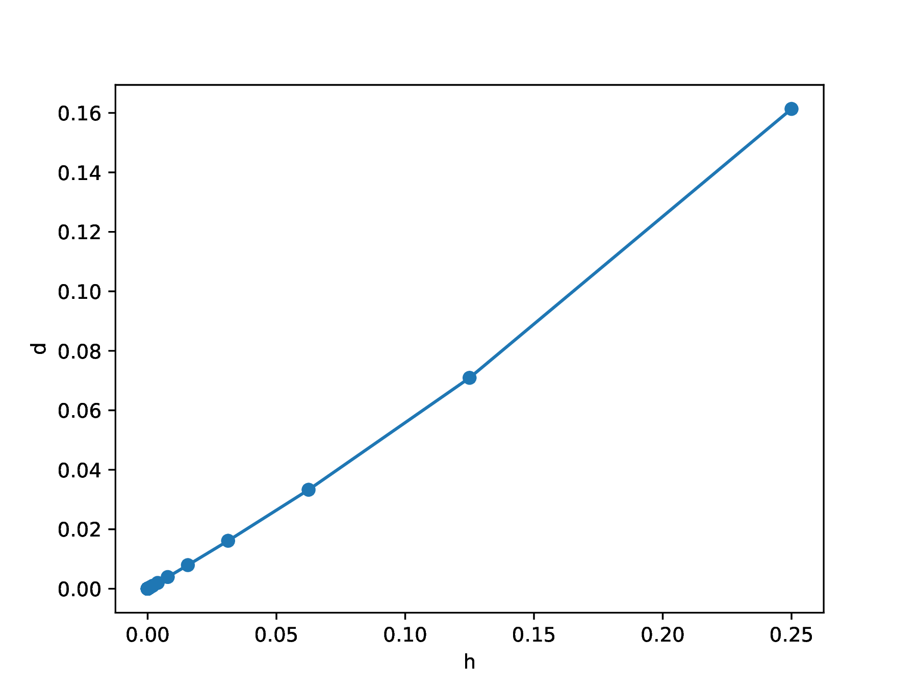
Investigation of the numerical results indicates increasing accuracy in the estimate of $g (x) = {(e^{x} - 1)}^{'} = e^{x}$ , $g (0) = 1$ with decreasing step size $h$ . The distance between successive approximation sequence terms $d_{n} = | g_{n} - g_{n - 1} |$ also decreases. It is more intuitive to analyze convergence behavior through a plot rather than a numerical table.

∴	clf(); plot(h[2:N],d,"-o"); xlabel("h"); ylabel("d");

∴	cd(homedir()*"//courses//MATH661//images"); savefig("L02Fig01a.eps");

∴

The intent of the rate and order of approximation definitions is to state that the distance between successive terms behaves as

d_{n + 1} ≅ s d_{n}^{q},

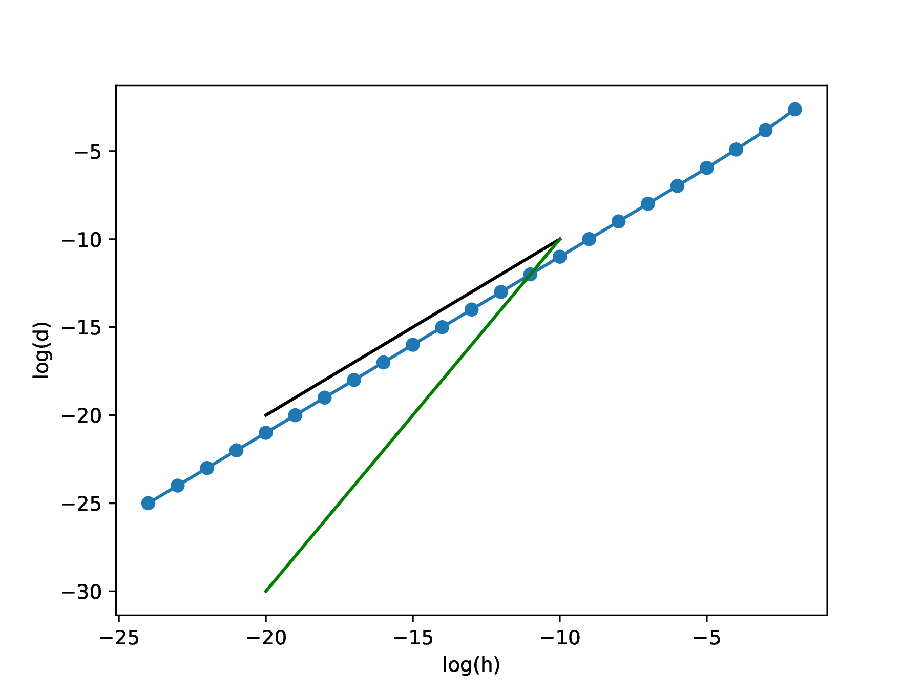
in the hope that this is a Cauchy sequence, and successively closer terms actually indicate convergence. The convergence parameters $(s, q)$ can be isolated by taking logarithms, $c_{n} = \log d_{n}$ leading to a linear dependence

c_{n + 1} ≅ q c_{n} + \log s .

Subtraction of successive terms gives $c_{n} - c_{n - 1} ≅ q (c_{n - 1} - c_{n - 2})$ , leading to an average slope estimate

q ≅ \frac{1}{N - 3} \sum_{n = 3}^{N - 1} \frac{c_{n} - c_{n - 1}}{c_{n - 1} - c_{n - 2}}

∴	c=log.(2,d); lh=log.(2,h[2:N]); clf(); plot(lh,c,"-o"); plot([-10,-20],[-10,-20],"k"); plot([-10,-20],[-10,-30],"g");

∴	xlabel("log(h)"); ylabel("log(d)"); savefig("L02Fig01b.eps");

∴	num=c[3:N-1]-c[2:N-2]; den=c[2:N-2]-c[1:N-3];

∴	q = sum(num ./ den)/(N-3)

$0.9920966582673338$

∴

The above computations indicate $q ≅ 1$ , known as linear convergence. Figure 1b shows the common practice of depicting guide lines of slope 1 (black) and slope 2 (green) to visually ascertain the rate of convergence. Once the order of approximation $q$ is determined, the rate of aproximation is estimated from

\log s ≅ \frac{1}{N - 2} \sum_{n = 2}^{N - 1} (c_{n} - q c_{n - 1}) .

∴	s=exp(sum(c[2:N-1]-q*c[1:N-2])/(N-2))

$0.3252477724180383$

∴

The above results suggest successive approximants become closer spaced according to

d_{n} ≅ 0.124 d_{n - 1}

Figure 1. (a, left). Convergence plot; (b,right) Convergence plot in logarithmic coordinates.

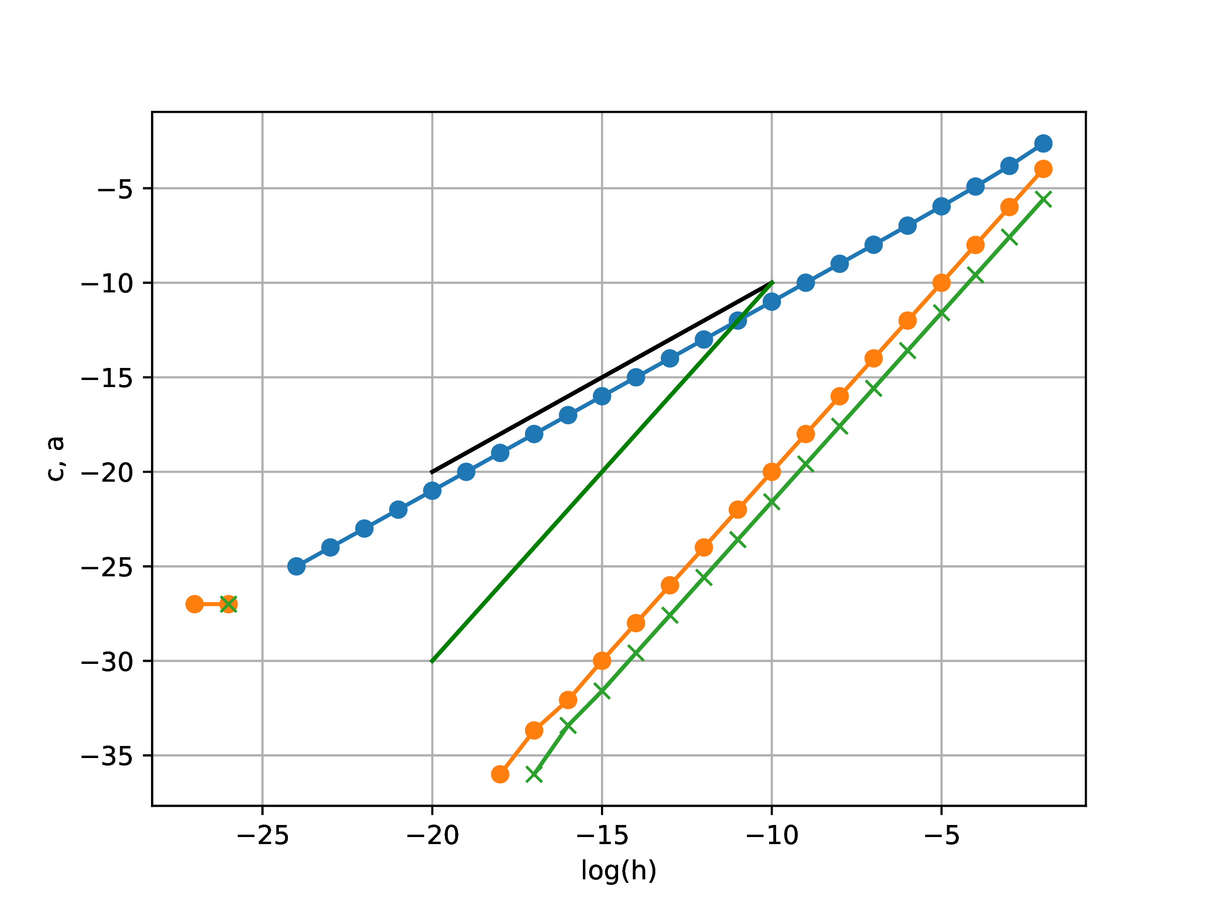
Repeat the above experiment at $x_{0} = \ln 2$ , where $g (\ln 2) = 2$ , and using a different approximation of the derivative

g_{n} = \frac{f (\ln 2 + h_{n}) - f (\ln 2 - h_{n})}{2 h_{n}} .

For this experiment, in addition to the rate and order of approximation $(s, q)$ , also determine the rate and order of convergence $(r, p)$ using

b_{n} = | g_{n} - g (π / 4) |, b_{n + 1} ≅ r b_{n}^{p}, a_{n} = \log b_{n}, a_{n + 1} = p a_{n} + \log r .

∴	N=32; n=1:N; h=2.0.^(-n); f(x) = exp(x)-1; x0=log(2); f0=f(x0); g0=exp(x0);

∴	g = (f.(x0 .+ h).-f.(x0 .- h)) ./ (2*h); d=abs.(g[2:N]-g[1:N-1]);

∴	c=log.(2,d); lh=log.(2,h[2:N]); b=abs.(g[2:N].-g0); a=log.(2,b);

∴	plot(lh,c,"-o"); plot(lh,a,"-x"); plot([-10,-20],[-10,-20],"k"); plot([-10,-20],[-10,-30],"g");

∴	xlabel("log(h)"); ylabel("c, a"); grid("on");

∴	savefig("L02Fig02.eps");

∴

Figure 2. Typical convergence behavior for approximants of a derivative. Blue line shows first-order or linear convergence of approximation $f^{'} (x_{0}) ≅ (f (x_{0} + h) - f (x_{0})) / h$ for $f (x) = e^{x} - 1$ at $x_{0} = 0$ . The convergence curve is monotone, with decreasing error for all sample points due to fortuitous $f (x_{0}) = 0$ . Green and orange lines indicate that the orders of convergence and approximation are quadratic for $f^{'} (x_{0}) ≅ (f (x_{0} + h) - f (x_{0} - h)) / (2 h)$ for $f (x) = e^{x} - 1$ at $x_{0} = \log 2$ . Now, $f (x_{0}) \neq 0$ , and small differences in the numerator are no longer resolved by the floating point system leading to an increase in the error for $\log (h) < - 20$ . The numerical experiment indicates that order of approximation can be used interchangeably with order of convergence, i.e., closer spacing of successive approximations is often an indication of convergence.

2.Convergence acceleration

Given some approximation sequence ${x_{n}}_{n \in ℕ}$ , $x_{n} \to x$ , with $x$ solution of problem $f (x) = 0$ , it is of interest to construct a more rapidly convergent sequence ${y_{n}}_{n \in ℕ}$ , $y_{n} \to x$ . Knowledge of the order of convergence $p$ can be used to achieve this purpose by writing

x_{n} - x ≅ r {(x_{n - 1} - x)}^{p}, x_{n - 1} - x ≅ r {(x_{n - 2} - x)}^{p},

(4)

and taking the ratio to obtain

\frac{x_{n} - x}{x_{n - 1} - x} = {(\frac{x_{n - 1} - x}{x_{n - 2} - x})}^{p} .

(5)

For $p \in ℕ$ , the above is a polynomial equation of degree $p$ that can be solved to obtain $x$ . The heuristic approximation (4) suggests a new approximation of the exact limit $x$ obtained by solving (5).

2.1.Aitken acceleration

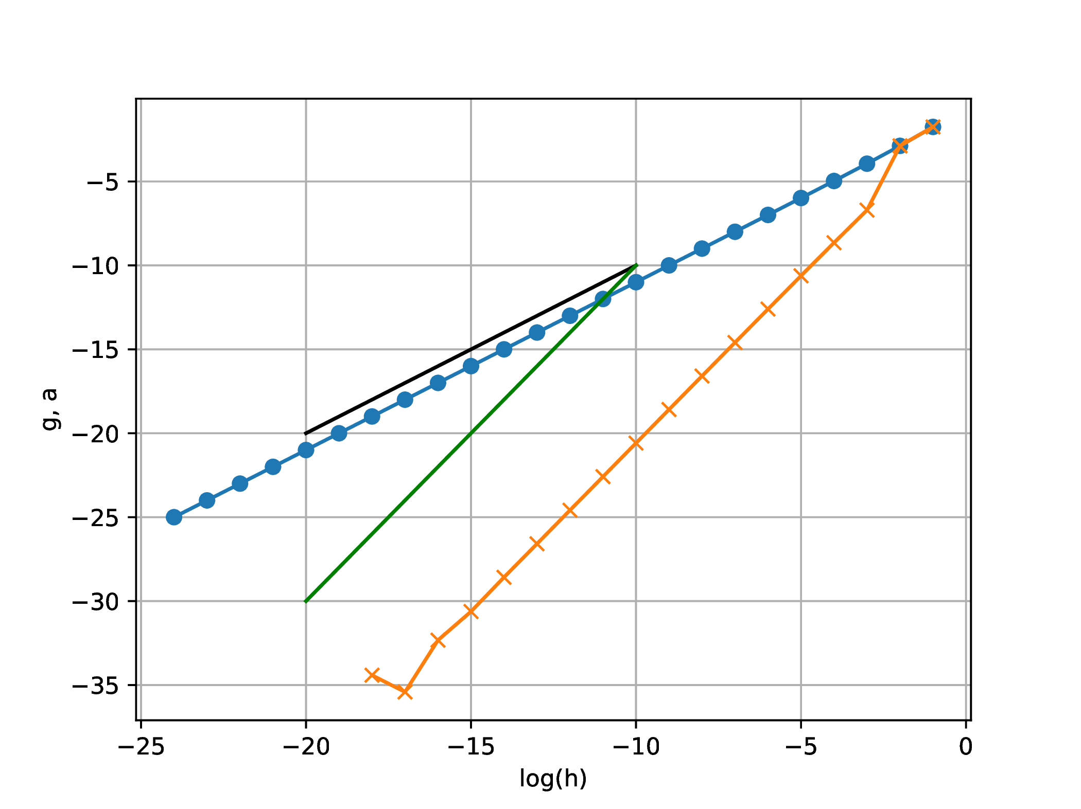
One of the widely used acceleration techniques was published by Aitken (1926, but had been in use since Medieval times) for $p = 1$ in which case (5) gives

x_{n} x_{n - 2} - (x_{n} + x_{n - 2}) x = x_{n - 1}^{2} - 2 x_{n - 1} x \Rightarrow x = \frac{x_{n} x_{n - 2} - x_{n - 1}^{2}}{x_{n} - 2 x_{n - 1} + x_{n - 2}} .

The above suggests that starting from ${x_{n}}_{n \in ℕ}$ , the sequence ${a_{n}}_{n \in ℕ}$ with

a_{n} = \frac{x_{n} x_{n - 2} - x_{n - 1}^{2}}{x_{n} - 2 x_{n - 1} + x_{n - 2}} = x_{n} - \frac{{(x_{n} - x_{n - 1})}^{2}}{x_{n} - 2 x_{n - 1} + x_{n - 2}},

might converge faster towards the limit. Investigate by revisiting the numerical experiment on approximation of the derivative $g = f^{'}$ of $f (x) = e^{x} - 1$ at $x_{0} = 0$ , using

g_{n} = \frac{f_{n} - f (0)}{h_{n}}, f_{n} = f (h_{n}), h_{n} = 2^{- n} .

∴	N=24; n=1:N; h=2.0.^(-n); f(x) = exp(x)-1; x0=0; f0=f(x0);

∴	g = (f.(h).-f0) ./ h; a = copy(g);

∴	a[3:N] = g[3:N] - (g[3:N]-g[2:N-1]).^2 ./ (g[3:N]-2*g[2:N-1]+g[1:N-2]);

∴	lh=log.(2,h); d=log.(2,abs.(g.-1)); b=log.(2,abs.(a.-1));

∴	clf(); plot(lh,d,"-o"); plot(lh,b,"-x"); plot([-10,-20],[-10,-20],"k"); plot([-10,-20],[-10,-30],"g"); xlabel("log(h)"); ylabel("g, a"); grid("on"); savefig("L02Fig03.eps");

∴

Figure 3. Aitken acceleration of linearly convergent sequence (blue dots) yields a close-to-quadratic convergent sequence (orange x).

Analysis reinforces the above numerical experiment. First-order convergence implies the distance to the limit decreases during iteration as

3.Approximation correction types

Several approaches may be used in construction of an approximating sequence ${x_{n}}_{n \in ℕ}$ . The approaches exemplified below for $x_{n} \in ℝ$ , can be generalized when $x_{n}$ is some other type of mathematical object.

3.1.Additive corrections

Returning to the Leibniz series

\frac{π}{4} = 1 - \frac{1}{3} + \frac{1}{5} - \frac{1}{7} + \frac{1}{9} - \dots .,

the sequence of approximations is ${L_{n}}_{n \in ℕ}$ with general term

L_{n} = \sum_{k = 0}^{n} \frac{{(- 1)}^{k}}{2 k + 1} .

Note that successive terms are obtained by an additive correction

L_{n} = L_{n - 1} + \frac{{(- 1)}^{n}}{2 n + 1}, L_{n} \to \frac{π}{4} .

Another example, again giving an approximation of $π$ is the Srinivasa Ramanujan series

R_{n} = \frac{2 \sqrt{2}}{9801} \sum_{k = 0}^{n} \frac{(4 k)! (1103 + 26390 k)}{{(k!)}^{4} 396^{4 k}}, {lim}_{n \to \infty} R_{n} = \frac{1}{π},

that can be used to obtain many digits of accuracy with just a few terms.

An example of the generalization of this approach is the Taylor series of a function. For example, the familiar sine power series

\sin x = x - \frac{x^{3}}{3!} + \frac{x^{5}}{5!} - \dots,

is analogous, but with rationals now replaced by monomials, and the limit is now a function $\sin : ℝ \to [- 1, 1]$ . The general term is

T_{n} (x) = \sum_{k = 0}^{n} \frac{{(- 1)}^{k} x^{2 k + 1}}{(2 k + 1)!},

and the same type of additive correction appears, this time for functions,

T_{n} (x) = T_{n - 1} (x) + \frac{{(- 1)}^{n} x^{2 n + 1}}{(2 n + 1)!}, T_{n} (x) \to \sin x .

3.2.Multiplicative corrections

Approximating sequences need not be constructed by adding a correction. Consider the approximation of $π / 2$ given by Wallis's product (1656)

S_{n} = (\frac{2}{1} \cdot \frac{2}{3}) \cdot (\frac{4}{3} \cdot \frac{4}{5}) \cdot (\frac{6}{5} \cdot \frac{6}{7}) \dots, S_{n} = \prod_{k = 1}^{n} \frac{4 k^{2}}{4 k^{2} - 1}, S_{n} \to \frac{π}{2},

for which

S_{n} = S_{n - 1} \cdot (\frac{4 n^{2}}{4 n^{2} - 1}) .

Another famous example is the Viète formula from 1593

\frac{2}{π} = \frac{\sqrt{2}}{2} \cdot \frac{\sqrt{2 + \sqrt{2}}}{2} \cdot \frac{\sqrt{2 + \sqrt{2 + \sqrt{2}}}}{2} \cdot \dots, V_{n} = \prod_{k = 1}^{n} \frac{\overset{k}{\underset{j = 1}{N}} \sqrt[2]{2}}{2}

in which the correction is multiplicative with numerators given by nested radicals. Similar to the $\sum$ symbol for addition, and the $\prod$ symbol for multiplication, the N symbol is used to denote nested radicals

\overset{k}{\underset{j = 1}{N}} \sqrt[b_{}]{a_{j}} = \sqrt[b_{1}]{a_{1} + \sqrt[b_{2}]{a_{2} + \sqrt[b_{3}]{a_{3} + \dots + \sqrt[b_{k}]{a_{k}}}}} .

In the case of the Viète formula, $a_{j} = 2$ , $b_{j} = 2$ for all $j$ .

3.3.Continued fractions

Yet another alternative is that of continued fractions, with one possible approximation of $π$ given by

π + 3 = 6 + \frac{1^{2}}{6 +} \frac{}{}

(6)

A notation is introduced for continued fractions using the $K$ symbol

F_{n} = b_{0} + \overset{n}{\underset{k = 1}{K}} \frac{a_{k}}{b_{k}} = b_{0} + \frac{a_{1}}{b_{1} +} .

Using this notation, the sequences arising in the continued fraction representation of $π$ are ${a_{n}}_{n \in ℕ}$ , ${b_{n}}_{n \in ℕ}$ chosen as $a_{k} = {(2 k - 1)}^{2}$ for $k \in ℕ_{+}$ , and $b_{k} = 6$ for $k \in ℕ$ .

π = {lim}_{n \to \infty} (6 + \overset{n}{\underset{k = 1}{K}} \frac{{(2 k - 1)}^{2}}{6}) .

3.4.Composite corrections

The above correction techniques used arithmetic operations. The repeated radical coefficients in the Viète formula suggest consideration of repeated composition of arbitrary functions $t_{0}, t_{1}, \dots, t_{n}$ to construct the approximant

insect

T_{n} = t_{0} \circ t_{1} \circ \dots \circ t_{n} = ⊙_{k = 0}^{n} t_{k} .

This is now a general framework, in which all of the preceeding correction approaches can be expressed. For example, the continued fraction formula (6) is recovered through the functions

t_{0} (z) = 6 + z, t_{1} (z) = \frac{1}{6 + z}, \dots, t_{k} (z) = \frac{{(2 k - 1)}^{2}}{6 + z},

and evaluation of the composite function at $z = 0$

F_{n} = T_{n} (0) .

This general framework is of significant current interest since such composition of nonlinear functions is the basis of deep neural network approximations.

Summary.

The cornerstone of scientific computing is construction of approximating sequences.
The problem of number approximation leads to definition of concepts and techniques that can be extended to more complex mathematical objects.
A primary objective is the construction of efficient approximating sequences, with efficiency characterized through concepts such as order and speed of convergence.
Though often enforced analytically, limiting behavior of the sequence is of secondary interest. As seen in the approximation of a derivative, the approximating sequence might diverge, yet give satisfactory answers for some range of indices.
Though by far the most widely studied and used approach to approximation, additive corrections are not the only possibility.
Alternative correction techniques include: multiplication, continued fractions, or repeated function composition.
Repeated composition of functions is used in constructing deep neural network approximants.