MATH661

Lecture 4: Linear Combinations

1.Finite-dimensional vector spaces

1.1.Overview

The definition from Table 1 of a vector space reflects everyday experience with vectors in Euclidean geometry, and it is common to refer to such vectors by descriptions in a Cartesian coordinate system. For example, a position vector $𝒓$ within the plane can be referred through the pair of coordinates $(x, y)$ . This intuitive understanding can be made precise through the definition of a vector space $ℛ_{2} = (ℝ^{2}, ℝ, +, \cdot)$ , called the real 2-space. Vectors within $ℛ_{2}$ are elements of $ℝ^{2} = ℝ \times ℝ = {(x, y) | . x, y \in ℝ}$ , meaning that a vector is specified through two real numbers, $𝒓 \leftrightarrow (x, y)$ . Addition of two vectors, $𝒒 \leftrightarrow (s, t)$ , $𝒓 \leftrightarrow (x, y)$ is defined by addition of coordinates $𝒒 + 𝒓 = (s + x, t + v)$ . Scaling $𝒓 \leftrightarrow (x, y)$ by scalar $a$ is defined by $a 𝒓 \leftrightarrow (a x, a y)$ . Similarly, consideration of position vectors in three-dimensional space leads to the definition of the $ℛ_{3} = (ℝ^{3}, ℝ, +, \cdot)$ , or more generally a real $m$ -space $ℛ_{m} = (ℝ^{m}, ℝ, +, \cdot)$ , $m \in ℕ$ , $m > 0$ .

Addition rules for	$\forall 𝒂, 𝒃, 𝒄 \in V$
$𝒂 + 𝒃 \in V$	Closure
$𝒂 + (𝒃 + 𝒄) = (𝒂 + 𝒃) + 𝒄$	Associativity
$𝒂 + 𝒃 = 𝒃 + 𝒂$	Commutativity
$𝟎 + 𝒂 = 𝒂$	Zero vector
$𝒂 + (- 𝒂_{}) = 𝟎$	Additive inverse
Scaling rules for	$\forall 𝒂, 𝒃 \in V$ , $\forall x, y \in S$
$x 𝒂 \in V$	Closure
$x (𝒂 + 𝒃) = x 𝒂 + x 𝒃$	Distributivity
$(x + y) 𝒂 = x 𝒂 + y 𝒂$	Distributivity
$x (y 𝒂) = (x y) 𝒂$	Composition
$1 𝒂 = 𝒂$	Scalar identity

Table 1. Vector space $𝒱 = (V, S, +, \cdot)$ properties for arbitrary $𝒂, 𝒃, 𝒄 \in V$

Note however that there is no mention of coordinates in the definition of a vector space as can be seen from the list of properties in Table 1. The intent of such a definition is to highlight that besides position vectors, many other mathematical objects follow the same rules. As an example, consider the set of all continuous functions $C (ℝ) = {f | . f : ℝ \to ℝ}$ , with function addition defined by the sum at each argument $t,$ $(f + g) (t) = f (t) + g (t)$ , and scaling by $a \in ℝ$ defined as $(a f) (t) = a f (t)$ . Read this as: “given two continuous functions $f$ and $g$ , the function $f + g$ is defined by stating that its value for argument $x$ is the sum of the two real numbers $f (t)$ and $g (t)$ ”. Similarly: “given a continuous function $f$ , the function $a f$ is defined by stating that its value for argument $t$ is the product of the real numbers $a$ and $f (t)$ ”. Under such definitions $𝒞^{0} = (C (ℝ), ℝ, +, \cdot)$ is a vector space, but quite different from $ℛ_{m}$ . Nonetheless, the fact that both $𝒞^{0}$ and $ℛ_{m}$ are vector spaces can be used to obtain insight into the behavior of continuous functions from Euclidean vectors, and vice versa. This correspondence principle between discrete and continuous formulations is a recurring theme in scientific computation.

1.2.Real vector space $ℛ_{m}$

Column vectors.

Since the real spaces

ℛ_{m} = (ℝ^{m}, ℝ, +, \cdot)

play such an important role in themselves and as a guide to other vector spaces, familiarity with vector operations in

ℛ_{m}

is necessary to fully appreciate the utility of linear algebra to a wide range of applications. Following the usage in geometry and physics, the

m

real numbers that specify a vector

𝒖 \in ℝ^{m}

are called the components of

𝒖

. The one-to-one correspondence between a vector and its components

𝒖 \leftrightarrow (u_{1}, \dots, u_{m})

, is by convention taken to define an equality relationship,

𝒖 = [\begin{array}{l} u_{1} \\ ⋮ \\ u_{m} \end{array}],

(1)

with the components arranged vertically and enclosed in square brackets. Given two vectors $𝒖, 𝒗 \in ℝ^{m}$ , and a scalar $a \in ℝ$ , vector addition and scaling are defined in $ℛ_{m}$ by real number addition and multiplication of components

$•$ $\circ$

𝒖 + 𝒗 = [\begin{array}{l} u_{1} \\ ⋮ \\ u_{m} \end{array}] + [\begin{array}{l} v_{1} \\ ⋮ \\ v_{m} \end{array}] = [\begin{array}{l} u_{1} + v_{1} \\ ⋮ \\ u_{m} + v_{m} \end{array}], a 𝒖 = a [\begin{array}{l} u_{1} \\ ⋮ \\ u_{m} \end{array}] = [\begin{array}{l} a u_{1} \\ ⋮ \\ a u_{m} \end{array}] .

(2)

∴	u=[1; 2; 3]; v=[-1; -2; -3]; [u v]

$[\begin{array}{cc} 1 & - 1 \\ 2 & - 2 \\ 3 & - 3 \end{array}]$ (3)

∴	a=2; b=5; au+bv

$[\begin{array}{c} - 3 \\ - 6 \\ - 9 \end{array}]$ (4)

∴

The vector space $ℛ_{m}$ is defined using the real numbers as the set of scalars, and constructing vectors by grouping together $m$ scalars, but this approach can be extended to any set of scalars $S$ , leading to the definition of the vector spaces $𝒮_{n} = (S^{n}, S, +, \cdot)$ . These will often be referred to as $n$ -vector space of scalars, signifying that the set of vectors is $V = S^{n}$ .

To aid in visual recognition of vectors, the following notation conventions are introduced:

vectors are denoted by lower-case bold Latin letters: $𝒖, 𝒗$ ;

scalars are denoted by normal face Latin or Greek letters: $a, b, α, β$ ;

the components of a vector are denoted by the corresponding normal face with subscripts as in equation (1);

related sets of vectors are denoted by indexed bold Latin letters: $𝒖_{1}, 𝒖_{2}, \dots, 𝒖_{n}$ .

Row vectors.

Instead of the vertical placement or components into one column, the components of could have been placed horizontally in one row

[\begin{array}{lll} u_{1} & \dots & u_{m} \end{array}]

, that contains the same data, differently organized. By convention vertical placement of vector components is the preferred organization, and

𝒖

shall denote a column vector henceforth. A transpose operation denoted by a

T

superscript is introduced to relate the two representations

$•$ $\circ$

𝒖^{T} = [\begin{array}{lll} u_{1} & \dots & u_{m} \end{array}],

∴	u=[1; 2; 3]; u'

$[\begin{array}{ccc} 1 & 2 & 3 \end{array}]$ (5)

∴

and $𝒖^{T}$ is the notation used to denote a row vector.

$•$ $\circ$ In Julia, horizontal placement of successive components in a row is denoted by a space.

∴

u=[4 5 6]

$[\begin{array}{ccc} 4 & 5 & 6 \end{array}]$ (6)

∴

Compatible vectors.

Addition of real vectors

𝒖, 𝒗 \in ℝ^{m}

defines another vector

𝒘 = 𝒖 + 𝒗 \in ℝ^{m}

. The components of

𝒘

are the sums of the corresponding components of

𝒖

and

𝒗

w_{i} = u_{i} + v_{i}

, for

i = 1, 2, \dots, m

. Addition of vectors with different number of components is not defined, and attempting to add such vectors produces an error. Such vectors with different number of components are called incompatible, while vectors with the same number of components are said to be compatible. Scaling of

𝒖

a

defines a vector

𝒛 = a 𝒖

, whose components are

z_{i} = a u_{i}

, for

i = 1, 2, \dots, m

1.3.Working with vectors

Ranges.

The vectors used in applications usually have a large number of components,

m ≫ 1

, and it is important to become proficient in their manipulation. Previous examples defined vectors by explicit listing of their

m

components. This is impractical for large

m

, and support is provided for automated generation for often-encountered situations. First, observe that Table 1 mentions one distinguished vector, the zero element that is a member of any vector space

𝟎 \in V

. The zero vector of a real vector space

ℛ_{m}

is a column vector with

m

components, all of which are zero, and a mathematical convention for specifying this vector is

𝟎^{T} = [\begin{array}{llll} 0 & 0 & \dots & 0 \end{array}] \in ℝ^{m}

. This notation specifies that transpose of the zero vector is the row vector with

m

zero components, also written through explicit indexing of each component as

𝟎_{i} = 0

, for

i = 1, \dots, m

. Keep in mind that the zero vector

𝟎

and the zero scalar

0

are different mathematical objects.

The ellipsis symbol in the mathematical notation is transcribed in Julia by the notion of a range, with 1:m denoting all the integers starting from $1$ to $m$ , organized as a row vector. The notation is extended to allow for strides different from one, and the mathematical ellipsis $i = m, m - 1, \dots, 1$ is denoted as m:-1:1. In general r:s:t denotes the set of numbers ${r, r + s, \dots, r + n s}$ with $r + n s ⩽ t$ , and $r, s, t$ real numbers and $n$ a natural number, $r, s, t \in ℝ$ , $n \in ℕ$ . If there is no natural number $n$ such that $r + n s ⩽ t$ , an empty vector with no components is returned.

2.Linear combinations

2.1.Linear combination as a matrix-vector product

The expression $𝒙 = x_{1} 𝒆_{1} + x_{2} 𝒆_{2} + \dots + x_{m} 𝒆_{m}$ expresses the idea of scaling vectors within a set and subsequent addition to form a new vector $𝒙$ . The matrix $𝑰 = [\begin{array}{llll} 𝒆_{1} & 𝒆_{2} & \dots & 𝒆_{m} \end{array}]$ groups these vectors together in a single entity, and the scaling factors are the components of the vector $𝒙$ . To bring all these concepts together it is natural to consider the notation

$•$ $\circ$

𝒙 = 𝑰 𝒙,

∴

UniformScaling{Bool}(true)

∴	Matrix(1I,3,3)

$[\begin{array}{ccc} 1 & 0 & 0 \\ 0 & 1 & 0 \\ 0 & 0 & 1 \end{array}]$ (7)

∴	Matrix(1.0I,3,3)

$[\begin{array}{ccc} 1.0 & 0.0 & 0.0 \\ 0.0 & 1.0 & 0.0 \\ 0.0 & 0.0 & 1.0 \end{array}]$ (8)

∴

as a generalization of the scalar expression $x = 1 \cdot x$ . It is clear what the operation $𝑰 𝒙$ should signify: it should capture the vector scaling and subsequent vector addition $x_{1} 𝒆_{1} + x_{2} 𝒆_{2} + \dots + x_{m} 𝒆_{m}$ . A specific meaning is now ascribed to $𝑰 𝒙$ by identifying two definitions to one another.

Linear combination.

Repeateadly stating “vector scaling and subsequent vector addition” is unwieldy, so a special term is introduced for some given set of vectors

{𝒂_{1}, \dots, 𝒂_{n}}

Definition. (Linear Combination) . The linear combination of vectors $𝒂_{1}, 𝒂_{2}, \dots, 𝒂_{n} \in V$ with scalars $x_{1}, x_{2}, \dots, x_{n} \in S$ in vector space $(V, S, +, \cdot)$ is the vector $𝒃 = x_{1} 𝒂_{1} + x_{2} 𝒂_{2} + \dots x_{n} 𝒂_{n} .$

Matrix-vector product.

Similar to the grouping of unit vectors

𝒆_{1}, \dots, 𝒆_{m}

into the identity matrix

𝑰

, a more concise way of referring to arbitrary vectors

𝒂_{1}, \dots, 𝒂_{n}

from the same vector space is the matrix

𝑨 = [\begin{array}{llll} 𝒂_{1} & 𝒂_{2} & \dots & 𝒂_{n} \end{array}]

. Combining these observations leads to the definition of a matrix-vector product.

Definition. (Matrix-Vector Product) . In the vector space $(V, S, +, \cdot)$ , the product of matrix $𝑨 = [\begin{array}{llll} 𝒂_{1} & 𝒂_{2} & \dots & 𝒂_{n} \end{array}]$ composed of columns $𝒂_{1}, 𝒂_{2}, \dots, 𝒂_{n} \in V$ with the vector $𝒙 \in S_{n}$ whose components are scalars $x_{1}, x_{2}, \dots, x_{n} \in S$ is the linear combination $𝒃 = x_{1} 𝒂_{1} + x_{2} 𝒂_{2} + \dots x_{n} 𝒂_{n} = 𝑨 𝒙 \in V .$

2.2.Linear algebra problem examples

Linear combinations in $E_{2}$ .

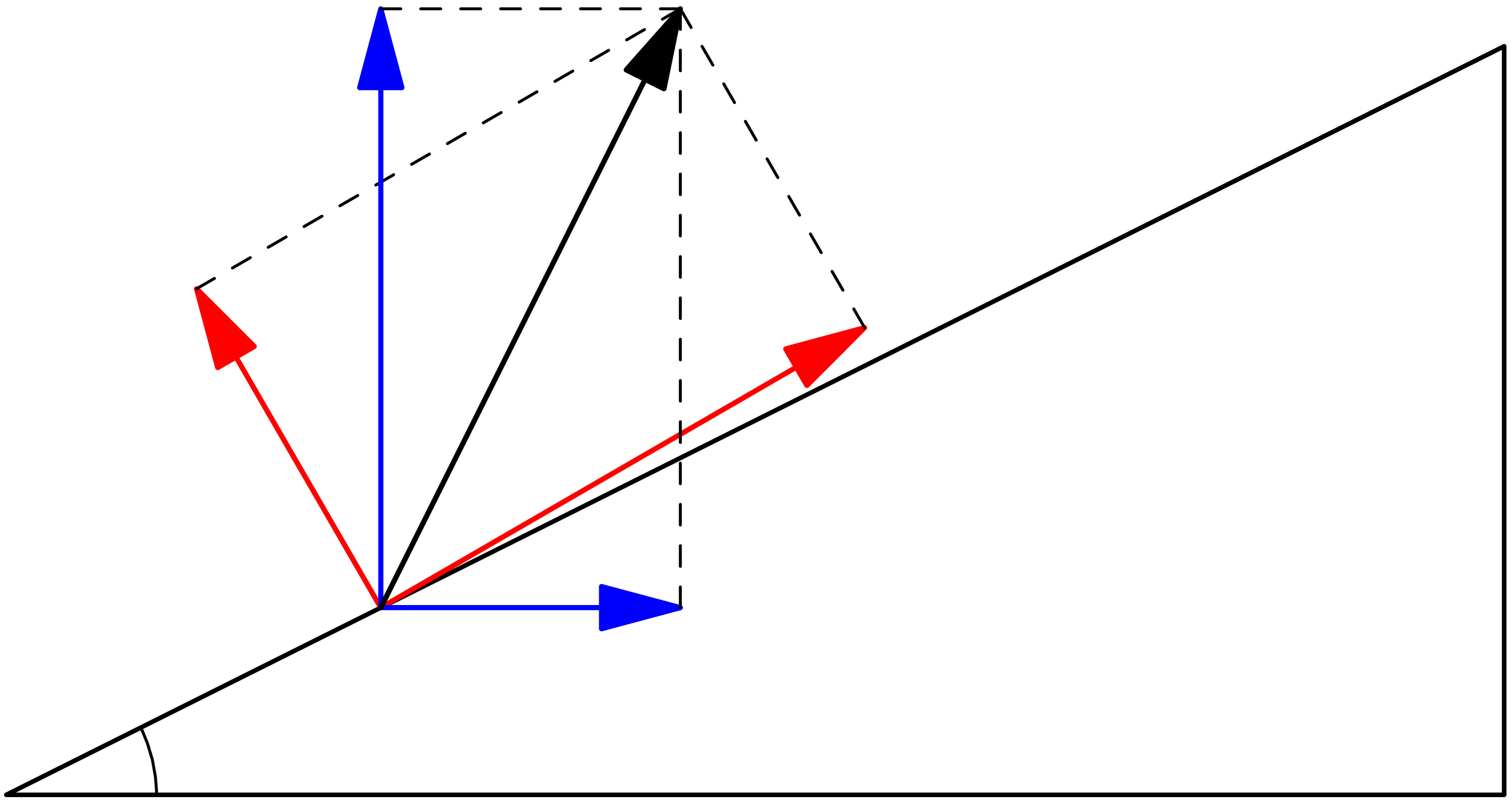
Consider a simple example that leads to a common linear algebra problem: decomposition of forces in the plane along two directions. Suppose a force is given in terms of components along the Cartesian

x, y

-axes,

𝒃 = b_{x} 𝒆_{x} + b_{y} 𝒆_{y}

, as expressed by the matrix-vector multiplication

𝒃 = 𝑰 𝒃 .

Note that the same force could be obtained by linear combination of other vectors, for instance the normal and tangential components of the force applied on an inclined plane with angle

θ

𝒃 = x_{t} 𝒆_{t} + x_{n} 𝒆_{n}

, as in Figure 1. This defines an alternate reference system for the problem. The unit vectors along these directions are

$•$ $\circ$

𝒕 = [\begin{array}{l} \cos θ \\ \sin θ \end{array}], 𝒏 = [\begin{array}{l} - \sin θ \\ \cos θ \end{array}],

∴	θ=π/6.; c=cos(θ); s=sin(θ); t=[c; s]; n=[-s; c];

∴

and can be combined into a matrix $𝑨 = [\begin{array}{ll} 𝒕 & 𝒏 \end{array}]$ . The value of the components $(x_{t}, x_{n})$ are the scaling factors and can be combined into a vector $𝒙 = {[\begin{array}{ll} x_{t} & x_{n} \end{array}]}^{T}$ . The same force must result irrespective of whether its components are given along the Cartesian axes or the inclined plane directions leading to the equality

$•$ $\circ$

𝑰 𝒃 = 𝒃 = 𝑨 𝒙 .

(9)

∴	b=[0.2; 0.4]; I*b

$[\begin{array}{c} 0.2 \\ 0.4 \end{array}]$ (10)

∴

Interpret equation (9) to state that the vector $𝒃$ could be obtained either as a linear combination of $𝑰$ , $𝒃 = 𝑰 𝒃$ , or as a linear combination of the columns of $𝑨$ , $𝒃 = 𝑨 𝒙$ . Of course the simpler description seems to be $𝑰 𝒃$ for which the components are already known. But this is only due to an arbitrary choice made by a human observer to define the force in terms of horizontal and vertical components. The problem itself suggests that the tangential and normal components are more relevant; for instance a friction force would be evaluated as a scaling of the normal force.

$•$ $\circ$ The components of $𝒃$ in this more natural reference system are not known, but can be determined by solving the vector equality $𝑨 𝒙 = 𝑰 𝒃 = 𝒃$ , known as a linear system of equations, implemented in many programming environments (Julia, Matlab, Octave) through the backslash operator x=A\b.

∴

A=[t n]

$[\begin{array}{cc} 0.8660254037844387 & - 0.49999999999999994 \\ 0.49999999999999994 & 0.8660254037844387 \end{array}]$ (11)

∴

x = A \ b

$[\begin{array}{c} 0.37320508075688774 \\ 0.2464101615137755 \end{array}]$ (12)

∴

[I*b A*x]

$[\begin{array}{cc} 0.2 & 0.2 \\ 0.4 & 0.4 \end{array}]$ (13)

∴

Figure 1. Alternative decompositions of force on inclined plane.

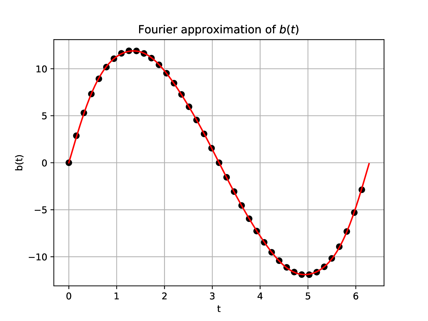
Linear combinations in $ℛ_{m}$ and $𝒞^{0} [0, 2 π)$ .

Linear combinations in a real space can suggest properties or approximations of more complex objects such as continuous functions. Let

𝒞^{0} [0, 2 π) = (C [0, 2 π), ℝ, +, \cdot)

denote the vector space of continuous functions that are periodic on the interval

[0, 2 π)

C [0, π) = {f | f : . ℝ \to ℝ, f (t) = f (t + 2 π)}

. Recall that vector addition is defined by

(f + g) (t) = f (t) + g (t)

, and scaling by

(a f) (t) = a f (t)

, for

f, g \in C [0, 2 π)

a \in ℝ

. Familiar functions within this vector space are

\sin (k t)

\cos (k t)

with

k \in ℕ

, and these can be recognized to intrinsically represent periodicity on

[0, 2 π)

, a role analogous to the normal and tangential directions in the inclined plane example. Define now another periodic function

b (t + 2 π) = b (t)

by repeating the values

b (t) = t (π - t) (2 π - t)

from the interval

[0, 2 π)

on all intervals

[2 p π, 2 (p + 1) π]

, for

p \in ℤ

. The function

b

is not given in terms of the “naturally” periodic functions

\sin (k t)

\cos (k t)

, but could it thus be expressed? This can be stated as seeking a linear combination

b (t) = \sum_{k = 1}^{\infty} x_{k} \sin (k t),

as studied in Fourier analysis. The coefficients

x_{k}

could be determined from an analytical formula involving calculus operations

x_{k} = \frac{1}{π} \int_{0}^{2 π} b (t) \sin (k t) d t,

but we'll seek an approximation using a linear combination of

n

terms

b (t) ≅ \sum_{k = 1}^{n} x_{k} \sin (k t), A (t) = [\begin{array}{llll} \sin (t) & \sin (2 t) & \dots & \sin (n t) \end{array}], A : ℝ \to ℝ^{n} .

Organize this as a matrix vector product $b (𝒕) ≅ A (𝒕) 𝒙$ , with

A (𝒕) = [\begin{array}{llll} \sin (𝒕) & \sin (2 𝒕) & \dots & \sin (n 𝒕) \end{array}], 𝒙 = {[\begin{array}{llll} x_{1} & x_{2} & \dots & x_{n} \end{array}]}^{T} \in ℝ^{n} .

The idea is to sample the column vectors of $A (𝒕)$ at the components of the vector $𝒕 = {[\begin{array}{llll} t_{1} & t_{2} & \dots & t_{m} \end{array}]}^{T} \in ℝ^{m}$ , $t_{j} = (j - 1) h$ , $j = 1, 2, \dots, m$ , $h = π / m$ . Let $𝒃 = b (𝒕)$ , and $𝑨 = A (𝒕)$ , denote the so-sampled $b, A$ functions leading to the definition of a vector $𝒃 \in ℝ^{m}$ and a matrix $𝑨 \in ℝ^{m \times n}$ . There are $n$ coefficients available to scale the column vectors of $𝑨$ , and $𝒃$ has $m$ components. For $m > n$ it is generally not possible to find $𝒙$ such that $𝑨 𝒙$ would exactly equal $𝒃$ , but as seen later the condition to be as close as possible to $𝒃$ leads to a well defined solution procedure. This is known as a least squares problem and is automatically applied in the x=A\b instruction when the matrix A is not square. As seen in the following numerical experiment and Figure 2, the approximation is excellent and the information conveyed by $m = 1000$ samples of $b (t)$ is now much more efficiently stored in the form chosen for the columns of $𝑨$ and the $n = 5$ scaling coefficients that are the components of $𝒙$ .

$•$ $\circ$

Figure 2. Comparison of least squares approximation (red line) with samples (black dots) of exact function $b (t) = t (π - t) (2 π - t)$

∴	m=1000; h=2*π/m; j=1:m;

∴	t=((j.-1)*h);

∴	n=3; A=sin.(t);

∴	for k=2:n global A A = [A sin.(k*t)] end;

∴	bt=t.(π.-t).(2*π.-t);

∴	x=A\bt; b=A*x;

∴	s=25; i=1:s:m; ts=t[i]; bs=bt[i];

∴	clf(); plot(ts,bs,"ok",t,b,"r");

∴	xlabel("t"); ylabel("b(t)"); grid("on")

∴	title("Fourier approximation of \$b(t)\$");

∴	cd(homedir()*"/courses/MATH661/images");

∴	savefig("L04Fig02.eps");

∴

Summary.

A widely used framework for constructing additive approximations is the vector space algebraic space structure in which scaling and addition operations are defined
In a vector space linear combinations are used to construct more complicated objects from simpler ones
$𝒃 = 𝑨 𝒙 = x_{1} 𝒂_{1} + \dots + x_{n} 𝒂_{n}$

Lecture 4: Linear Combinations

1.Finite-dimensional vector spaces

1.1.Overview

1.2.Real vector space ℛm

Column vectors.

Row vectors.

Compatible vectors.

1.3.Working with vectors

Ranges.

2.Linear combinations

2.1.Linear combination as a matrix-vector product

Linear combination.

Matrix-vector product.

2.2.Linear algebra problem examples

Linear combinations in E2.

Linear combinations in ℛm and 𝒞0[0,2π).

Summary.

1.2.Real vector space $ℛ_{m}$

Linear combinations in $E_{2}$ .

Linear combinations in $ℛ_{m}$ and $𝒞^{0} [0, 2 π)$ .