Lecture 8: Least Squares Approximation

A typical scenario in many sciences is acquisition of $m$ numbers to describe some object that is understood to actually require only $n\ll m$ parameters. For example, $m$ voltage measurements $u_i$ of an alternating current could readily be reduced to three parameters, the amplitude, phase and frequency $u\left(t\right)=a\sin (\omega t+\phi )$. Very often a simple first-degree polynomial approximation $y=ax+b$ is sought for a large data set $D=\{(x_i,y_i),i=1,\dots ,m\}$. All of these are instances of data compression, a problem that can be solved in a linear algebra framework.

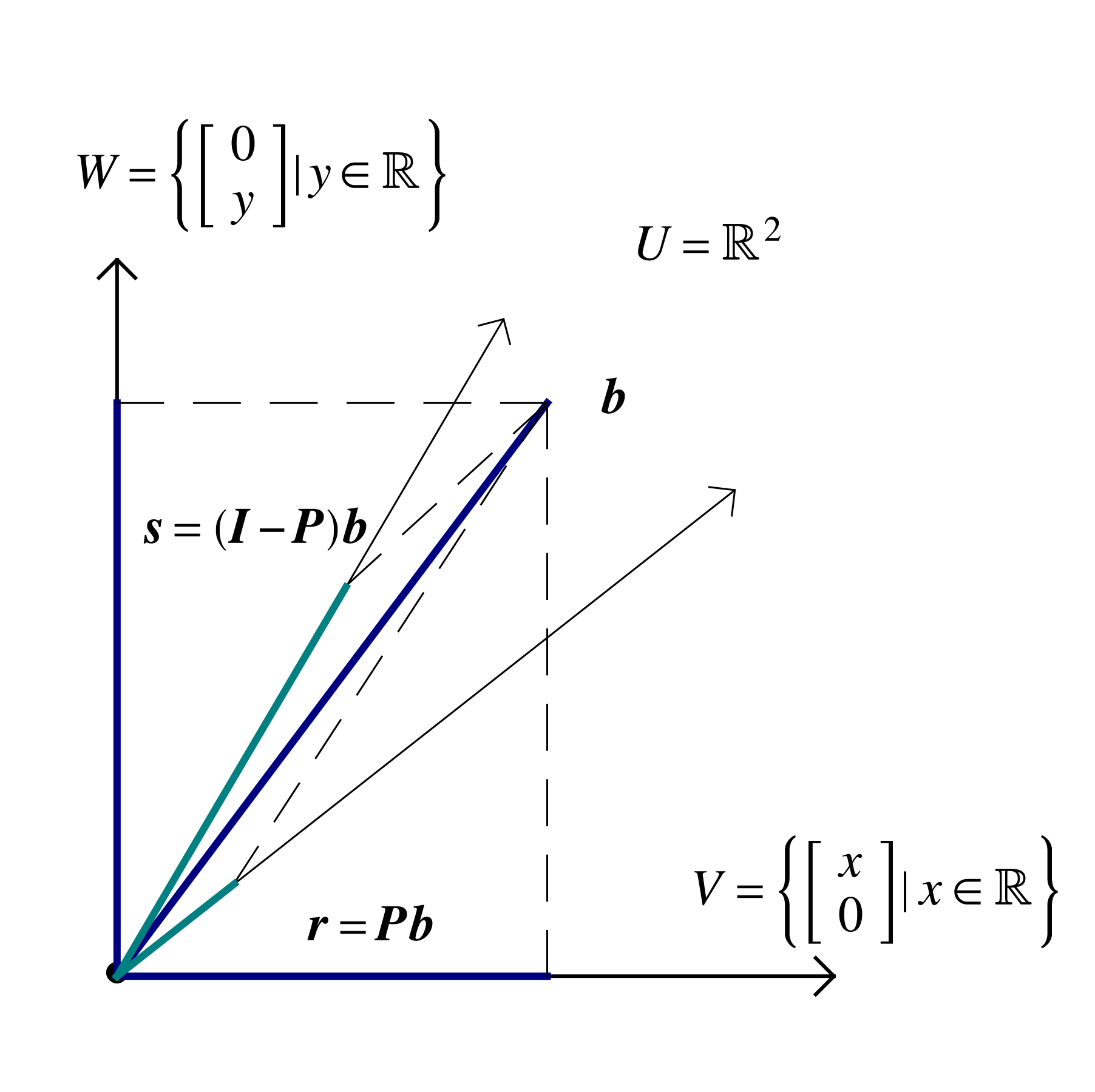
Consider a partition of a vector space $U$ into orthogonal subspaces $U=V\oplus W$, $V=W^{\perp }$, $W=V^{\perp }$. Within the typical scenario described above $U={ℝ}^m$, $V\subset {ℝ}^m$, $W\subset {ℝ}^m$, $\dim V=n$, $\dim W=m-n$. If $𝑽=\left[\begin{array}{ccc}{𝒗}_1& \dots & {𝒗}_n\end{array}\right]\in {ℝ}^{m\times n}$ is a basis for $V$ and $𝑾=\left[\begin{array}{ccc}{𝒘}_1& \dots & {𝒘}_{m-n}\end{array}\right]\in {ℝ}^{m\times (m-n)}$ is a basis for W, then $𝑼=\left[\begin{array}{cccccc}{𝒗}_1& \dots & {𝒗}_n& {𝒘}_1& \dots & {𝒘}_{m-n}\end{array}\right]$ is a basis for $U$. Even though the matrices $𝑽,𝑾$ are not necessarily square, they are said to be orthonormal, in the sense that all columns are of unit norm and orthogonal to one another. Computation of the matrix product ${𝑽}^T𝑽$ leads to the formation of the identity matrix within ${ℝ}^n$

Similarly, ${𝑾}^T𝑾={𝑰}_{m-n}$. Whereas for the square orthogonal matrix $𝑼$ multiplication both on the left and the right by its transpose leads to the formation of the identity matrix

the same operations applied to rectangular orthonormal matrices lead to different results

A simple example is provided by taking $𝑽={𝑰}_{m,n}$, the first $n$ columns of the identity matrix in which case

∴ 

I4=1.0*I(4); V=I4[:,1:2]; P=V*V'

∴ 

Q=I4-P; b=rand(4,1); r=P*b; s=Q*b; [P b r s]

∴ 

Figure 1. Projection in ${ℝ}^2$. The vectors $𝒓,𝒔\in {ℝ}^2$ have two components, but could be expressed through scaling of ${𝒆}_1,{𝒆}_2$.

Returning to the general case, the orthogonal matrices $𝑼\in {ℝ}^{m\times m}$, $𝑽\in {ℝ}^{m\times n}$, $𝑾\in {ℝ}^{m\times (m-n)}$ are associated with linear mappings $𝒃=𝒇\left(𝒙\right)=𝑼𝒙$, $𝒓=𝒈\left(𝒃\right)=𝑷𝒃$, $𝒔=𝒉\left(𝒃\right)=(𝑰-𝑷)𝒃$. The mapping $𝒇$ gives the components in the $𝑰$ basis of a vector whose components in the $𝑼$ basis are $𝒙$. The mappings $𝒈,𝒉$ project a vector onto span$\{{𝒗}_1,\dots ,{𝒗}_n\}$, span$\{{𝒘}_1,\dots ,{𝒘}_{m-n}\}$, respectively. When $𝑽,𝑾$ are orthogonal matrices the projections are also orthogonal $𝒓\perp 𝒔$. Projection can also be carried out onto nonorthogonal spanning sets, but the process is fraught with possible error, especially when the angle between basis vectors is small, and will be avoided henceforth.

Notice that projection of a vector already in the spanning set simply returns the same vector, which leads to a general definition.

Definition. The mapping is called a projection if $𝒇\circ 𝒇=𝒇$, or if for any $𝒖\in U$, $𝒇\left(𝒇\left(𝒖\right)\right)=𝒇\left(𝒖\right)$. With $𝑷$ the matrix associated $𝒇$, a projection matrix satisfies ${𝑷}^2=𝑷$.

2.Gram-Schmidt

Orthonormal vector sets $\{{𝒒}_1,\dots ,{𝒒}_n\}$ are of the greatest practical utility, leading to the question of whether some such a set can be obtained from an arbitrary set of vectors $\{{𝒂}_1,\dots ,{𝒂}_n\}$. This is possible for independent vectors, through what is known as the Gram-Schmidt algorithm

1. Start with an arbitrary direction ${𝒂}_1$

2. Divide by its norm to obtain a unit-norm vector ${𝒒}_1={𝒂}_1/||{𝒂}_1||$

3. Choose another direction ${𝒂}_2$

4. Subtract off its component along previous direction(s) ${𝒂}_2-\left({𝒒}_1^T{𝒂}_2\right){𝒒}_1$

5. Divide by norm ${𝒒}_2=({𝒂}_2-\left({𝒒}_1^T{𝒂}_2\right){𝒒}_1)/||{𝒂}_2-\left({𝒒}_1^T{𝒂}_2\right){𝒒}_1||$

6. Repeat the above

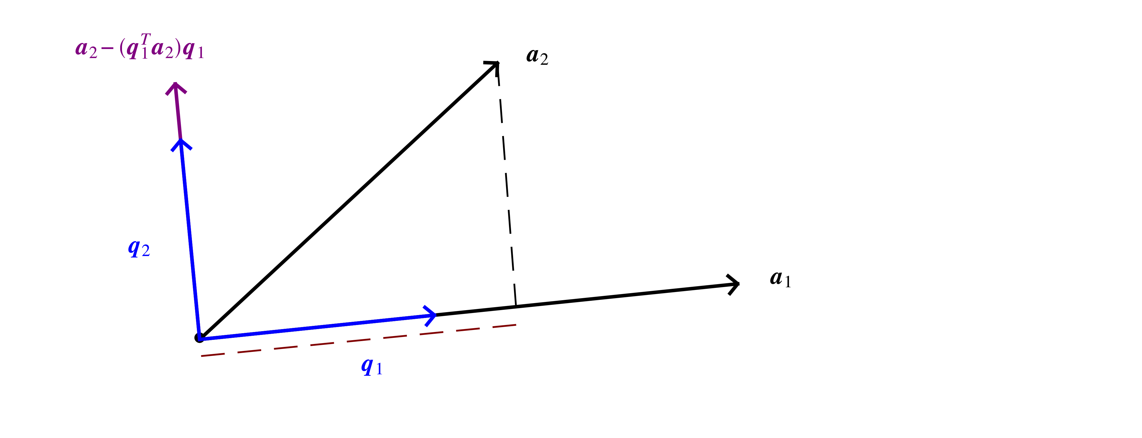
The above geometrical description can be expressed in terms of matrix operations as

equivalent to the system

The system is easily solved by forward substitution resulting in what is known as the (modified) Gram-Schmidt algorithm, transcribed below both in pseudo-code and in Julia.

∴ 

function mgs(A)
  m,n=size(A); Q=copy(A); R=zeros(n,n)
  for i=1:n
    R[i,i]=sqrt(Q[:,i]'*Q[:,i])
    if (R[i,i]<eps())
      break
    end
    Q[:,i]=Q[:,i]/R[i,i]
    for j=i+1:n
      R[i,j]=Q[:,i]'*A[:,j]
      Q[:,j]=Q[:,j]-R[i,j]*Q[:,i]
    end
  end
  return Q,R
end;

∴ 

∴ 

A=rand(3,3); Q,R=mgs(A); Q

∴ 

Q1,R1=qr(A); Q

∴ 

By analogy to arithmetic and polynomial algebra, the Gram-Schmidt algorithm furnishes a factorization

with $𝑸\in {ℝ}^{m\times n}$ with orthonormal columns and $𝑹\in {ℝ}^{n\times n}$ an upper triangular matrix, known as the $QR$-factorization. Since the column vectors within $𝑸$ were obtained through linear combinations of the column vectors of $𝑨$ we have

3.$QR$ solution of linear algebra problems

The $QR$-factorization can be used to solve basic problems within linear algebra.

3.1.Transformation of coordinates

Recall that when given a vector $𝒃\in {ℝ}^m$, an implicit basis is assumed, the canonical basis given by the column vectors of the identity matrix $𝑰\in {ℝ}^{m\times m}$. The coordinates $𝒙$ in another basis $𝑨\in {ℝ}^{m\times m}$ can be found by solving the equation

by an intermediate change of coordinates to the orthogonal basis $𝑸$. Since the basis $𝑸$ is orthogonal the relation ${𝑸}^T𝑸=𝑰$ holds, and changes of coordinates from $𝑰$ to $𝑸$, $𝑸𝒄=𝒃,$ are easily computed $𝒄={𝑸}^T𝒃$. Since matrix multiplication is associative

the relations $𝑹𝒙={𝑸}^T𝒃=𝒄$ are obtained, stating that $𝒙$ also contains the coordinates of $𝒄$ in the basis $𝑹$. The three steps are:

1. Compute the $QR$-factorization, $𝑸𝑹=𝑨$;

2. Find the coordinates of $𝒃$ in the orthogonal basis $𝑸$, $𝒄={𝑸}^T𝒃$;

3. Find the coordinates of $𝒙$ in basis $𝑹$, $𝑹𝒙=𝒄$.

Since $𝑹$ is upper-triangular,

the coordinates of $𝒄$ in the $𝑹$ basis are easily found by back substitution.

∴ 

function bcks(R,c)
  m,n=size(R); x=zeros(m,1)
  for i=m:-1:1
    x[i]=c[i]/R[i,i]
    for j=i-1:-1:1
      c[j]=c[j]-R[j,i]*x[i]
    end
  end
  return x
end;

∴ 

∴ 

xex=rand(3,1); b=A*xex; Q,R=mgs(A); c=Q'*b;

∴ 

x=bcks(R,c); x0=A\b; [xex x0]

∴ 

3.2.General orthogonal bases

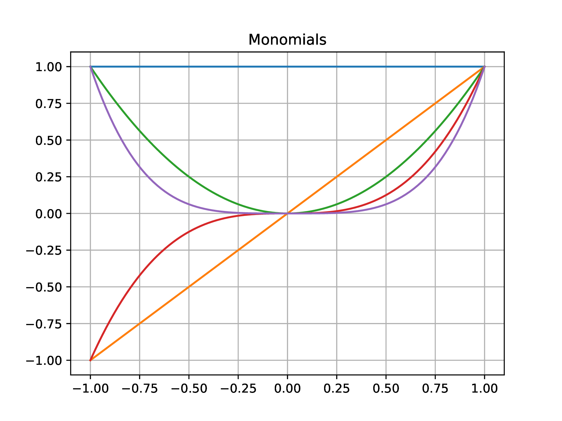
The above approch for the real vector space ${ℛ}_m$ can be used to determine orthogonal bases for any other vector space by appropriate modification of the scalar product. For example, within the space of smooth functions ${𝒞}^{\infty }[-1,1]$ that can differentiated an arbitrary number of times, the Taylor series

is seen to be a linear combination of the monomial basis $𝑴=\left[\begin{array}{cccc}1& x& x^2& \dots \end{array}\right]$ with scaling coefficients ${\{f\left(0\right),f^{\text{'}}\left(0\right),\frac{1}{2}{f}^{\text{'}\text{'}}\left(0\right),\dots \}}^{}$. The scalar product

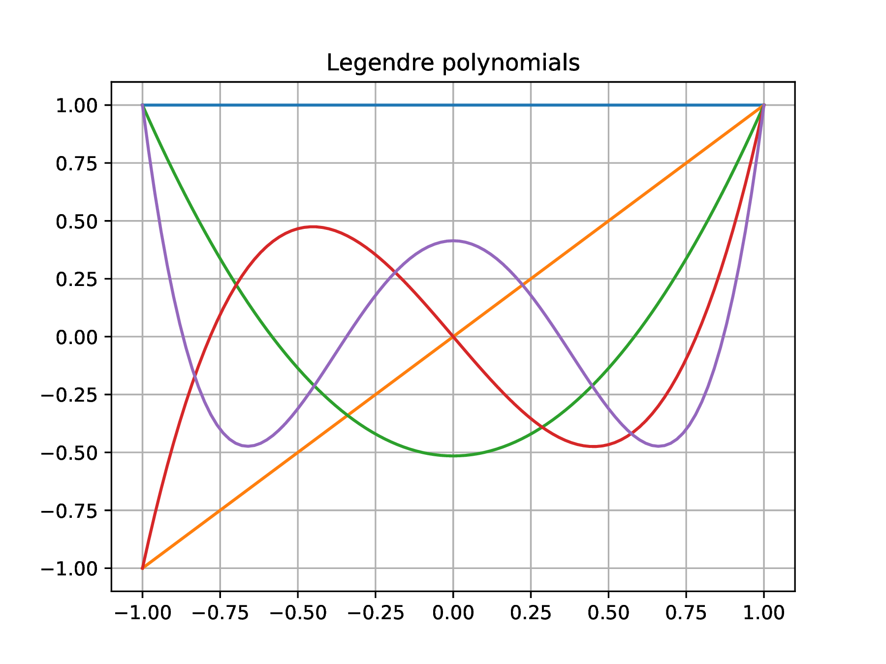
can be seen as the extension to the $[-1,1]$ continuum of a the vector dot product. Orthogonalization of the monomial basis with the above scalar product leads to the definition of another family of polynomials, known as the Legendre polynomials

∴ 

m=101; h=2.0/(m-1); x=(0:m-1)*h .- 1.0;

∴ 

M=[x.^0 x.^1 x.^2 x.^3 x.^4]; Q,R=mgs(M);

∴ 

S=diagm(1.0 ./ Q[m,:]); P=Q*S; sc=[-1 1 -1 1];

∴ 

figure(1); clf(); plot(x,M[:,1],x,M[:,2],x,M[:,3],x,M[:,4],x,M[:,5]);

∴ 

grid("on"); title("Monomials"); savefig("images/monomials.eps");

∴ 

figure(2); clf(); plot(x,P[:,1],x,P[:,2],x,P[:,3],x,P[:,4],x,P[:,5]);

∴ 

grid("on"); title("Legendre polynomials");

∴ 

savefig("images/LegendrePolynomials.eps");

∴ 

3.3.Least squares

The approach to compressing data $D=\left\{(x_i,y_i)|i=1,\dots ,m.\right\}$ suggested by calculus concepts is to form the sum of squared differences between $y\left(x_i\right)$ and $y_i$, for example for $y\left(x\right)=a_0+a_{1}x$ when carrying out linear regression,

and seek $(a_0,a_1)$ that minimize $S(a_0,a_1)$. The function $S(a_0,a_1)⩾0$ can be thought of as the height of a surface above the $a_0{a}_1$ plane, and the gradient $\nabla S$is defined as a vector in the direction of steepest slope. When at some point on the surface if the gradient is different from the zero vector $\nabla S\ne 𝟎$, travel in the direction of the gradient would increase the height, and travel in the opposite direction would decrease the height. The minimal value of $S$ would be attained when no local travel could decrease the function value, which is known as stationarity condition, stated as $\nabla S=0$. Applying this to determining the coefficients $(a_0,a_1)$ of a linear regression leads to the equations

The above calculations can become tedious, and do not illuminate the geometrical essence of the calculation, which can be brought out by reformulation in terms of a matrix-vector product that highlights the particular linear combination that is sought in a liner regression. Form a vector of errors with components $e_i=y\left(x_i\right)-y_i$, which for linear regression is $y\left(x\right)=a_0+a_{1}x$. Recognize that $y\left(x_i\right)$ is a linear combination of $1$ and $x_i$ with coefficients $a_0,a_1$, or in vector form

The norm of the error vector $||𝒆||$ is smallest when $𝑨𝒂$ is as close as possible to $𝒚$. Since $𝑨𝒂$ is within the column space of $C\left(𝑨\right)$, $𝑨𝒂\in C\left(𝑨\right)$, the required condition is for $𝒆$ to be orthogonal to the column space

The above is known as the normal system, with $𝑵={𝑨}^T𝑨$ is the normal matrix. The system $𝑵𝒂=𝒃$ can be interpreted as seeking the coordinates in the $𝑵={𝑨}^T𝑨$ basis of the vector $𝒃={𝑨}^T𝒚$. An example can be constructed by randomly perturbing a known function $y\left(x\right)=a_0+a_{1}x$ to simulate measurement noise and compare to the approximate $\stackrel{\sim }{𝒂}$ obtained by solving the normal system.

1. Generate some data on a line and perturb it by some random quantities

   ∴	m=100; x=LinRange(0,1,m); a=[2; 3];

   ∴	a0=a[1]; a1=a[2]; yex=a0 .+ a1*x; y=(yex+rand(m,1) .- 0.5);

   ∴

2. Form the matrices $𝑨$, $𝑵={𝑨}^T𝑨$, vector $𝒃={𝑨}^T𝒚$

   ∴	A=ones(m,2); A[:,2]=x; N=A'*A; b=A'*y;

   ∴

3. Solve the system $𝑵𝒂=𝒃$, and form the linear combination $\stackrel{\sim }{𝒚}=𝑨𝒂$ closest to $𝒚$

   ∴	atilde=N\b; [a atilde]

   ${\displaystyle \left[\begin{array}{cc}2.0& 1.9215699010834906\\ 3.0& 3.03714411616737\end{array}\right]}$

   (6)

   ∴

The normal matrix basis $𝑵={𝑨}^T𝑨$ can however be an ill-advised choice. Consider $𝑨\in {ℝ}^{2\times 2}$ given by

where the first column vector is taken from the identity matrix ${𝒂}_1={𝒆}_1$, and second is the one obtained by rotating it with angle $\theta$. If $\theta =\pi /2$, the normal matrix is orthogonal, ${𝑨}^T𝑨=𝑰$, but for small $\theta$, $𝑨$ and $𝑵={𝑨}^T𝑨$ are approximated as

When $\theta$ is small ${𝒂}_1,{𝒂}_2$ are almost colinear, and ${𝒏}_1,{𝒏}_2$ even more so. This can lead to amplification of small errors, but can be avoided by recognizing that the best approximation in the 2-norm is identical to the Euclidean concept of orthogonal projection. The orthogonal projector onto $C\left(𝑨\right)$ is readily found by $QR$-factorization, and the steps to solve least squares become

1. Compute $𝑸𝑹=𝑨$

2. The projection of $𝒚$ onto the column space of $𝑨$ is $𝒛=𝑸{𝑸}^T𝒚$, and has coordinates $𝒄={𝑸}^T𝒚$ in the orthogonal basis $𝑸$.

3. The same $𝒛$ can also obtained by linear combination of the columns of $𝑨$, $𝒛=𝑨𝒂=𝑸{𝑸}^T𝒚$, and replacing $𝑨$ with its $QR$-factorization gives $𝑸𝑹𝒂=𝑸𝒄$, that leads to the system $𝑹𝒂=𝒄$, solved by back-substitution.

∴ 

Q,R=mgs(A); c=Q'*y;

∴ 

aQR=R\c; [a atilde aQR]

∴ 

The above procedure carried over to approximation by higher degree polynomials.

∴ 

m=100; n=6; x=LinRange(0,1,m); a=rand(-10:10,n,1); A=ones(m,1);

∴ 

for j=1:n-1
  global A
  A = [A x.^j];
end

∴ 

yex=A*a; y=yex .+ 0.001*(rand(m,1) .- 0.5); N=A'*A;

∴ 

b=A'*y;

∴ 

atilde=N\b; Q,R=mgs(A); c=Q'*y;

∴ 

aQR=R\c; [a atilde aQR]

∴