MATH661

Stabilized Orthogonal Factorizations

1.Conditioning of linear algebra problems

Recall that the relative condition number of a mathematical problem $f : X \to Y$ characterizes the amplification by $f$ of perturbations in its argument

κ = {lim}_{ε \to 0} {sup}_{|| δ x || ⩽ ε} (\frac{|| f (x + δ x) - f (x) ||}{|| f (x) ||} / \frac{|| δ x ||}{|| x ||}) .

Linear combination. The basic operation of linear combination $𝑨 𝒙$ , $𝑨 \in ℂ^{m \times n}$ , seen as the problem $ℂ^{n} \overset{𝒇}{\to} ℂ^{m}$ has the condition number

κ = {sup}_{δ x} (\frac{|| 𝑨 δ 𝒙 ||}{|| 𝑨 𝒙 ||} / \frac{|| δ 𝒙 ||}{|| 𝒙 ||}) = {sup}_{δ x} (\frac{|| 𝑨 δ 𝒙 ||}{|| δ 𝒙 ||}) \frac{|| 𝒙 ||}{|| 𝑨 𝒙 ||} = || 𝑨 || \frac{|| 𝒙 ||}{|| 𝑨 𝒙 ||} .

The matrix norm property $|| 𝑨 𝒚 || ⩽ || 𝑨 || || 𝒚 ||$ can be used to obtain

|| 𝒙 || = || 𝑰_{n} 𝒙 || = || 𝑨^{+} 𝑨 𝒙 || ⩽ || 𝑨^{+} || || 𝑨 𝒙 || \Rightarrow \frac{|| 𝒙 ||}{|| 𝑨 𝒙 ||} ⩽ || 𝑨^{+} ||

leading to

κ ⩽ || 𝑨^{} || || 𝑨^{+} || = κ (𝑨),

where $κ (𝑨)$ is the condition number of the matrix $𝑨$ . If $𝑨$ is of full rank with $m > n$ , the 2-norm condition number is given by the ratio of largest to smallest singular values.

|| 𝑨 || = σ_{1}, || 𝑨^{+} || = 1 / σ_{n} \Rightarrow κ (𝑨) = σ_{1} / σ_{n} ⩾ 1 .

By convention, if $𝑨$ is singular, the condition number $κ (𝑨) = \infty$ .

Coordinate transformation. For $𝑨 \in ℂ^{m \times m}$ of full rank, the coordinates of vector $𝒃 \in ℂ^{m}$ expressed in the $𝑰$ basis can be transformed its coordinates $𝒙 \in ℂ^{m}$ in the $𝑨$ basis by solving the linear system $𝑨 𝒙 = 𝑰 𝒃$ , with the solution $𝒙 = 𝑨^{- 1} 𝒃$ (so written formally, even though the inverse is almost never explicitly computed). This is simply another linear combination of the columns of $𝑨^{- 1}$ , hence the problem $𝒇 : ℂ^{m} \to C^{m}$ , $𝒇 (𝒃) = 𝑨^{- 1} 𝒃$ again has a condition number bounded by the condition number of the matrix $𝑨$ .

κ ⩽ || 𝑨^{- 1} || || 𝑨 || = κ (𝑨) = κ (𝑨^{- 1}) .

Operator perturbation. Instead of changing the input data as above, the linear mapping represented by the matrix $𝑨 \in ℂ^{m \times n}$ might itself be perturbed. Two mathematical problems may now be formulated:

For fixed $𝒃 \in ℂ^{m}, 𝒇 : ℂ^{m \times n} \to ℂ^{n}, 𝒇 (𝑨, 𝒃) = 𝑨^{+} 𝒃 = 𝒙$ . Perturbation of the input $𝑨$ induces perturbation of $𝒙$ in order for $𝒃$ to be kept fixed
$(𝑨 + δ 𝑨) (𝒙 + δ 𝒙) = 𝒃 .$
Using $𝑨 𝒙 = 𝒃$ , and assuming that $δ 𝑨 δ 𝒙$ is negligible gives
$𝑨 δ 𝒙 + δ 𝑨 𝒙 = 𝟎 \Rightarrow δ 𝒙 = - 𝑨^{+} δ 𝑨 𝒙,$
hence the relative condition number is
$κ = \frac{|| 𝑨^{+} δ 𝑨 𝒙 ||}{|| 𝒙 ||} \cdot \frac{|| 𝑨 ||}{|| δ 𝑨 ||} ⩽ \frac{|| 𝑨^{+} || || δ 𝑨 𝒙 ||}{|| 𝒙 ||} \cdot \frac{|| 𝑨 ||}{|| δ 𝑨 ||} ⩽ \frac{|| 𝑨^{+} || || δ 𝑨 || || 𝒙 ||}{|| 𝒙 ||} \cdot \frac{|| 𝑨 ||}{|| δ 𝑨 ||} = κ (𝑨) .$

For all above linear algebra problems the condition number is bounded by the associated matrix condition number. Unitary matrices $𝑸 \in ℂ^{m \times m}$ have $κ (𝑸) = 1$ , and define an orthonormal basis for $ℂ^{m}$ . A rank-deficient matrix $𝒁 \in ℂ^{m \times m}$ has $κ (𝒁) = \infty$ , and corresponds to a linearly dependent vector set ${𝒛_{1}, \dots, 𝒛_{m}}$ . The behavior of many numerical approximation procedures based upon linear combinations is determined by condition number of the basis set.

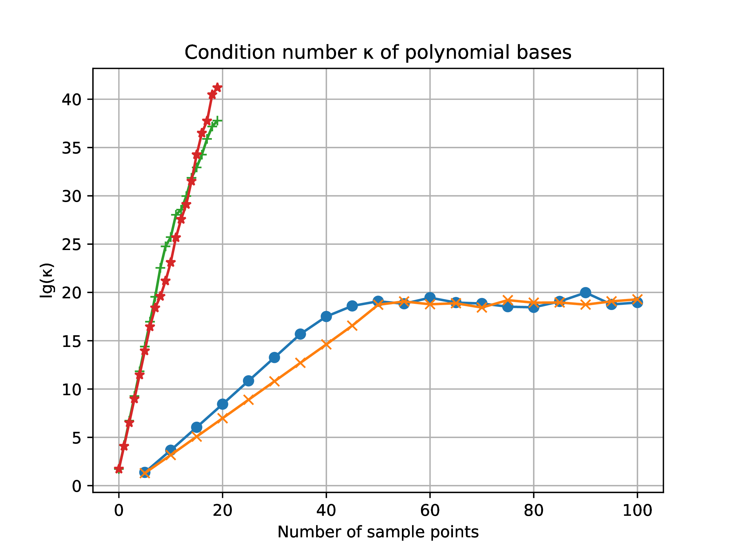
$•$ Monomial basis with uniform sampling. Sampling the monomial basis on interval $[a, b]$ at $t_{i} = i h + a, i = 0, m$ , $h = (b - a) / (m - 1)$ leads to the Vandermonde matrix

𝑽 = [\begin{array}{llll} 𝟏 & 𝒕 & \dots & 𝒕^{m} \end{array}],

an extremely ill-conditioned matrix (Fig. ). This can readily be surmised from the example $a = 0$ , $b = 1$ , in which case for large $m$ the last columns of $𝑽$ become ever more colinear to the same $𝒆_{m}$ vector. Series expansions based on the monomials such as the Taylor series

f (t) = f (0) + f^{'} (0) t + \dots + \frac{f^{(n)} (0)}{n!} t^{n} + \dots

are highly sensitive to pertubations, small changes in $f (t)$ lead to large changes in the coordinates ${f (0), f^{'} (0), \dots}$ .

∴	function Vandermonde(a,b,m) t=LinRange(a,b,m); v=ones(m,1); V=copy(v) for j=2:m v = v .* t; V=[V v] end return V end;

∴

$•$ Monomial basis with Chebyshev sampling. Changing the sampling so that points are clustered towards the interval endpoints reduces the condition number at fixed number of sampling points $m$ , but the same limiting behavior for large $m$ is obtained.

∴	function VandermondeC(m) δ=π/(2m); ϴ=LinRange(δ,π-δ,m) t=cos.(ϴ) v=ones(m,1); V=copy(v) for j=2:m v = v . t; V=[V v] end return V end;

∴

$•$ Triangular basis with uniform sampling. $L U$ -factorization of the monomial basis leads to a different family of polynomials, known as a triangular basis

{1, t - x_{1}, (t - x_{1}) \cdot (t - x_{2}), \dots, (t - x_{1}) \cdot \dots \cdot (t - x_{m - 1})},

where ${x_{1}, \dots, x_{m}}$ are known as the nodes of the system. These can be chosen to uniformly sample an interval. As to be expected, applying a sequence of non-unitary linear transformations onto an ill-conditioned basis yields even worse conditioning.

∴	function Triangular(a,b,m) x=LinRange(a,b,m); T=ones(m,1); Tj=copy(T); t=copy(x) for j=2:m Tj = Tj .* (t .- x[j-1]); T=[T Tj] end return T end;

∴

$\circ$ Triangular basis with Chebyshev sampling. Adopting Chebyshev sampling ameliorates the conditioning, but only marginally.

$\circ$

Figure 1. Monomial basis with: (o) uniform sampling, (x) Chebyshev sampling. Triangular basis with: (+) uniform sampling, (*) Chebyshev sampling.

∴	mr=5:5:100; κVDMU=log10.(cond.(Vandermonde.(-1,1,mr)));

∴	κVDMC=log10.(cond.(VandermondeC.(mr)));

∴	κTU=log10.(cond.(Triangular.(-1,1,mr)));

∴	κTC=log10.(cond.(TriangularC.(mr)));

∴

∴	x=collect(mr); clf();

∴	plot(x,κVDMU,"o-",x,κVDMC,"x-",κTU,"+-",κTC,"*-");

∴	grid("on"); title("Condition number κ of polynomial bases");

∴	xlabel("Number of sample points"); ylabel("lg(κ)");

∴	pre="/home/student/courses/MATH661/images/";

∴	savefig(pre*"PolyBasesCondNr.eps");

∴

2.Orthogonal factorization through Householder reflectors

The Gram-Schmidt procedure constructs an orthogonal factorization by linear combinations of the column vectors of $𝑨 \in ℂ^{m \times n}$ , $m ⩾ n$ , $rank (𝑨) = n$

𝑨 𝑹_{1} 𝑹_{2} \dots 𝑹_{n} = 𝑸 \Rightarrow 𝑨 = 𝑸 𝑹, 𝑹 = 𝑹_{n}^{- 1} \dots 𝑹_{1}^{- 1} .

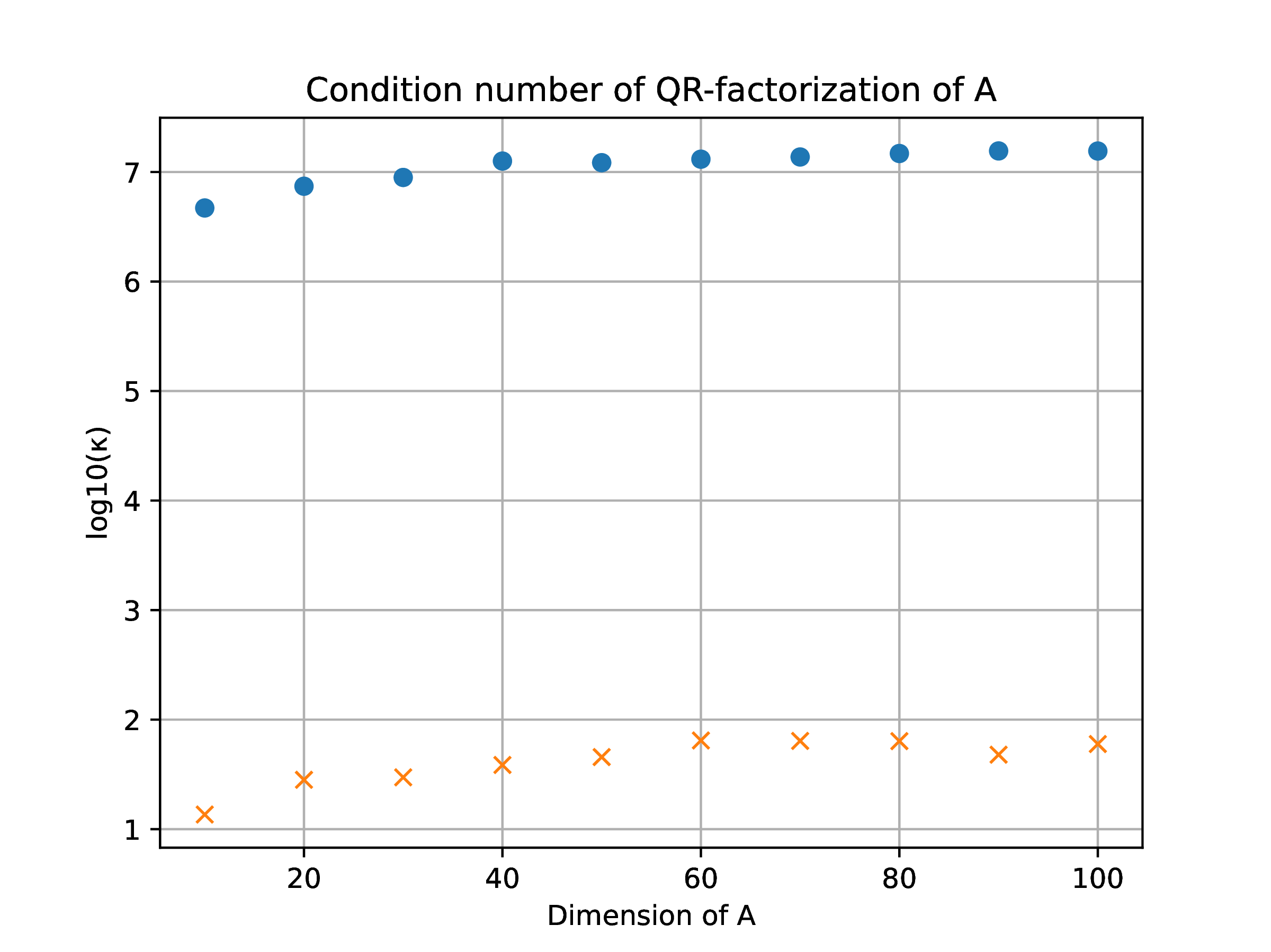
In exact arithmetic $C (𝑸) = C (𝑨)$ by construction, and $κ (𝑸) = 1$ , but the sequence of multiplications with $𝑹_{1}, \dots, 𝑹_{n}$ might amplify perturbations in $𝑨$ (due for example to floating point representation errors or inherent uncertainty in knowledge of $𝑨$ ). The problem $𝒇 : ℂ^{m \times n} \to C^{m \times n} \times ℂ^{n \times n},$ $𝑨 \overset{𝒇}{\to} 𝑸, 𝑹$ has condition number

κ = \frac{|| δ 𝑸 ||}{|| 𝑸 ||} \cdot \frac{|| 𝑨 ||}{|| δ 𝑨 ||} + \frac{|| δ 𝑹 ||}{|| 𝑹 ||} \cdot \frac{|| 𝑨 ||}{|| δ 𝑨 ||},

and numerical experimentation (Fig. 2) readily exhibits large condition numbers.

An alternative approach is to obtain an orthogonal factorization through unitary transformations

𝑸_{n} \dots 𝑸_{1} 𝑨 = 𝑹 \Rightarrow 𝑨 = 𝑸 𝑹, 𝑸 = 𝑸_{1}^{*} \dots 𝑸_{n}^{*} .

Unitary transformations do not modify vector 2-norms or relative orientations

{|| 𝑸 𝒙 ||}^{2} = 𝒙^{*} 𝑸^{*} 𝑸 𝒙 = {|| 𝒙 ||}^{2}, {(𝑸 𝒚)}^{*} (𝑸 𝒙) = 𝒚^{*} 𝒙,

and are hence said to be isometric. In Euclidean space reflections and rotations are isometric.

$\circ$

Figure 2. $Q R$ -conditioning: (o) modified Gram-Schmidt, (x) Householder.

Estimation of the $Q R$ -condition number by numerical experimentation: generate $N$ random perturbations of a matrix, compute the factorization of each perturbed matrix, and choose the maximum encountered value as $κ$ .

∴

function mgs(A)
  m,n=size(A); Q=copy(A); R=zeros(n,n)
  for i=1:n
    R[i,i]=sqrt(Q[:,i]'*Q[:,i])
    if (R[i,i]<eps())
      break
    end
    Q[:,i]=Q[:,i]/R[i,i]
    for j=i+1:n
      R[i,j]=Q[:,i]'*A[:,j]
      Q[:,j]=Q[:,j]-R[i,j]*Q[:,i]
    end
  end
  return Q,R
end;

∴

function QRcondGS(N,A,ε)
  Q,R=mgs(A); κ=1; normA=norm(A); normR=norm(R)
  for k=1:N
    δA=ε*randn(size(A))
    δF=qr(A+δA); δQ=Array(δF.Q)-Q; δR=Array(δF.R)-R
    κ = max(κ, (norm(δQ)+norm(δR)/normR)*normA/norm(δA) )
  end
  return κ
end;

∴	mr=10:10:100; κQRGS = log10.(QRcondGS.(100,randn.(mr,mr),1.0e-6));

∴	x=collect(mr); clf(); plot(x,κQRGS,"o");

∴

∴

function QRcond(N,A,ε)
  F=qr(A); Q=Array(F.Q); R=Array(F.R)
  κ=1; normA=norm(A); normR=norm(R)
  for k=1:N
    δA=ε*randn(size(A))
    δF=qr(A+δA); δQ=Array(δF.Q)-Q; δR=Array(δF.R)-R
    κ = max(κ, (norm(δQ)+norm(δR)/normR)*normA/norm(δA) )
  end
  return κ
end;

∴	κQR = log10.(QRcond.(100,randn.(mr,mr),1.0e-6));

∴	x=collect(mr); plot(x,κQR,"x");

∴	grid("on"); title("Condition number of QR-factorization of A");

∴	xlabel("Dimension of A"); ylabel("log10(κ)");

∴	savefig(pre*"QRcond.eps");

∴

Construction of an isometric reflection transformation suitable for a $Q R$ factorization is represented in Fig. 3. Let vector $𝒙 \in ℂ^{m + 1 - k}$ represent the portion of the $k^{th}$ column from the diagonal downwards in stage $k$ of reduction of $𝑨 \in ℂ^{m \times n}$ to upper triangular form

𝑸_{k - 1} \dots 𝑸_{1} 𝑨 = [\begin{array}{ll} 𝑹_{} & 𝑪 \\ 𝟎 & 𝑩 \end{array}], 𝑩 = [\begin{array}{llll} 𝒙 & 𝒃_{2} & \dots & 𝒃_{n - k} \end{array}] .

The next stage of in reduction to upper triangular form is the isometric transformation of $𝒙$ into $\pm || 𝒙 || 𝒆_{1}$ , with $𝒆_{1} \in ℂ^{m + 1 - k}$ the unit vector along the first direction. With $𝒗 = \pm || 𝒙 𝒆_{1} || - 𝒙$ , $𝒒 = 𝒗 / || 𝒗 ||$ , the projection of $𝒙$ onto the span of $𝒗$ , $C (𝒗)$ is

𝒚 = 𝑷_{𝒗} 𝒙 = 𝒒 𝒒^{*} 𝒙,

and its complementary projector onto $N (𝒗^{*})$ is

𝒛 = 𝑷_{⊥ 𝒗} = (𝑰 - 𝒒 𝒒^{*}) 𝒙 .

The reflector transforming $𝒙$ into $\pm || 𝒙 || 𝒆_{1}$ is obtained by doubling the above displacements, and is known as a Householder reflector

𝑯 = 𝑰 - 2 𝒒 𝒒^{*} .

Of the two possibilities $\pm || 𝒙 || 𝒆_{1}$ , the choice

𝒗 = - sign (x_{1}) || 𝒙 || 𝒆_{1} - 𝒙,

avoids loss of floating accuracy $𝒙 ≅ || 𝒙 || 𝒆_{1}$ . For $𝒙 \in ℂ^{m + 1 - k}$ , $sign (x_{1}) = \exp (\arg (x_{1}))$ .

Figure 3. Geometry of Householder reflector

The resulting Householder $Q R$ -factorization is given

Input: $𝑨 \in ℂ^{m \times n}$

$𝑸 = 𝟎_{m, n}$

for $k = 1 : n$

$𝒙 = 𝑨 [k : m, k]$

$𝒗 = sign (x_{1}) || 𝒙 || + 𝒙$

$𝒒 = 𝒗 / || 𝒗 ||$ ; $𝑸 [k : m, k] = 𝒒$

for $j = k : n$

$𝑨 [k : m, j] = 𝑨 [k : m, j] - 2 𝒒 (𝒒^{*} 𝑨 [k : m, j])$

∴

function HouseholderQR(A)
  m,n=size(A)
  Q=zeros(m,n); R=copy(A)
  for k=1:n
    x=R[k:m,k]
    e1=zeros(size(x)); e1[1]=1
    v=sign(x[1])*norm(x)*e1+x
    q=v/norm(v); Q[k:m,k]=q
    for j=k:n
      aj=R[k:m,j]; c=2*q'*aj
      R[k:m,j]=aj.-c*q
    end
  end
  return Q,R
end;

∴

Note that the above implementation does not return the $𝑸$ matrix, but rather the $𝑸_{1}, \dots, 𝑸_{n}$ reflectors from which $𝑸$ can be reconstructed if needed. Usually though, the $𝑸$ matrix itself is not required, but rather the product $𝑸 𝒖$ which can readily be evaluated as $𝑸_{n} \dots 𝑸_{1} 𝒖$ . The Householder reflector algorithm is typically the default procedure in $Q R$ -factorizations implemented in software systems, and as seen in (Fig. 2), leads to much better conditioning.

3.Orthogonal factorization through Given rotators

An alternative approach to orthogonal factorization utilizes isometric rotation transformations of the form

𝑹 (i, k, θ) = 𝑰 + (\cos θ - 1) (𝒆_{i} 𝒆_{i}^{*} + 𝒆_{k} 𝒆_{k}^{*}) - \sin θ (𝒆_{i} 𝒆_{k}^{*} - 𝒆_{k} 𝒆_{i}^{*}),

with the rotation angle $θ$ chosen to nullify the subdiagonal element $(i, k)$ , $i > k$

{(𝑹 (i, k, θ) 𝑨)}_{i k} = a_{k k} \sin θ + a_{i k} \cos θ = 0 \Rightarrow θ_{i k} = \arctan (- \frac{a_{i k}}{a_{k k}}) .

Composition of repeated rotations $𝑸_{i k} = 𝑹 (i, k, θ_{i k})$ can be organized to lead to an upper triangular matrix

𝑸_{m n} \dots 𝑸_{32} 𝑸_{m 1} \dots 𝑸_{31} 𝑸_{21} 𝑨 = 𝑹 .

Whereas Householder reflectors work on entire vectors, Givens rotators nullify individual subdiagonal elements. For full matrices Householder reflectors typically require fewer floating point operations, but the special structure of a sparse matrix is better exploited by use of Givens rotators.

Input: $𝑨 \in ℂ^{m \times n}$

$𝑸 = 𝟎_{m, n}$

for $k = 1 : n$

for $i = k + 1 : m$

$θ = \arctan (- a_{i k} / a_{k k})$

$c = \cos (θ)$ ; $s = \sin (θ)$

for $j = k : n$

$u = a_{k j}$ ; $v = a_{i j}$

$a_{k j} = c u - s v$

$a_{i j} = s u + c v$

∴

function GivensQR(A)
  m,n=size(A)
  Q=zeros(m,n); R=copy(A)
  for k=1:n
    for i=k+1:m
      θ = atan(-R[i,k],R[k,k]); Q[i,k]=
      c = cos(θ); s = sin(θ)
      for j=k:n
        u = R[k,j]; v = R[i,j]
        R[k,j]=c*u-s*v
        R[i,j]=s*u+c*v
      end
    end
  end
  return Q,R
end;

∴

As in the Householder implementation the above implementation returns data to reconstruct $𝑸$ if needed.