MATH661

1.Interpolation error

As mentioned, a polynomial interpolant of $f : ℝ \to ℝ$ already incorporates the function values $y_{i} = f (x_{i}), i = 0, \dots, n$ , so additional information on $f$ is required to estimate the error

e (t) = f (t) - p (t),

when $t$ is not one of the sample points. One approach is to assume that $f$ is smooth, $f \in C^{\infty} (ℝ)$ , in which case the error is given by

f (t) - p (t) = \frac{f^{(n + 1)} (ξ_{t})}{(n + 1)!} \prod_{i = 0}^{n} (t - x_{i}) = \frac{f^{(n + 1)} (ξ_{t})}{(n + 1)!} w (t),

(1)

for some $ξ_{t} \in [x_{0}, x_{n}]$ , assuming $x_{0} < x_{1} < \dots < x_{n}$ . The above error estimate is obtained by repeated application of Rolle's theorem to the function

Φ (u) = f (u) - p (u) - \frac{f (t) - p (t)}{w (t)} w (u),

that has $n + 1$ roots at $t, x_{0}, x_{1}, \dots, x_{n}$ , hence its $(n + 1)$ -order derivative must have a root in the interval $(x_{0}, x_{n})$ , denoted by $ξ_{t}$

Φ^{(n + 1)} (ξ_{t}) = \frac{d^{n + 1} Φ}{d u^{n + 1}} (ξ_{t}) = 0 = f^{(n + 1)} (ξ_{t}) - \frac{f (t) - p (t)}{w (t)} (n + 1)!,

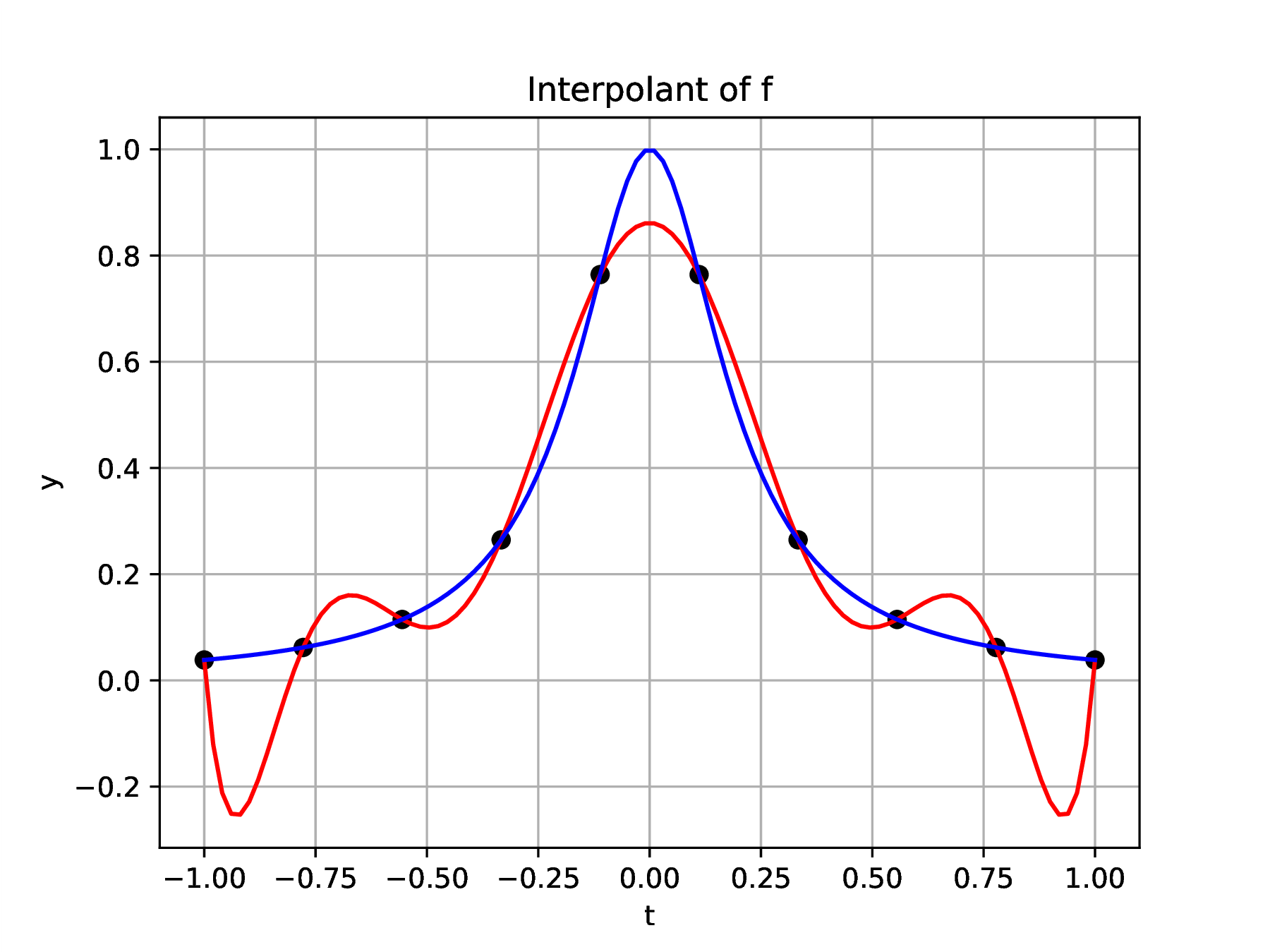
establishing (1.2). Though the error estimate seems promising due to the $(n + 1)!$ in the denominator, the derivative $f^{(n + 1)}$ can be arbitrarily large even for a smooth function. This is the behavior that arises in the Runge function $f (t) = 1 / [1 + {(5 t)}^{2}]$ (Fig. 1), for which a typical higher-order derivative appears as

$\circ$

f^{(10)} = \frac{35437500000000 (107421875 t^{10} - 64453125 t^{8} + 7218750 t^{6} - 206250 t^{4} + 1375 t^{2} - 1)}{{(25 t^{2} + 1)}^{11}}, {|| f^{(10)} ||}_{\infty} ≅ 3.5 \times 10^{13} .

In[29]:=

Runge[t_]=1/(1+25*t^2); Simplify[D[Runge[t],{t,10}]]

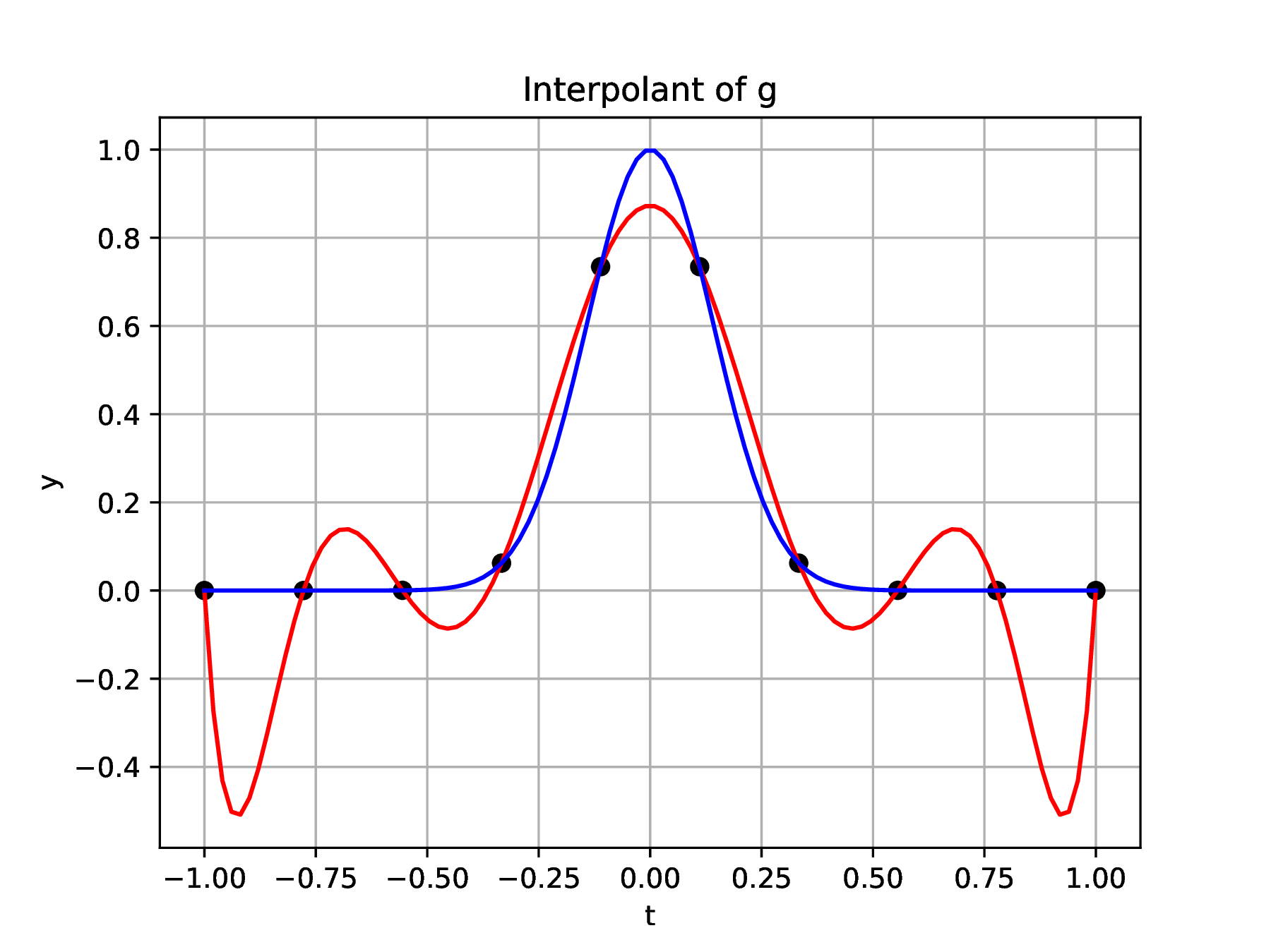
$\frac{35437500000000 (107421875 t^{10} - 64453125 t^{8} + 7218750 t^{6} - 206250 t^{4} + 1375 t^{2} - 1)}{{(25 t^{2} + 1)}^{11}}$

In[30]:=

The behavior might be attributable to the presence of poles of $f$ in the complex plane at $t_{1, 2} = \pm i / 5$ , but the interpolant of the holomorphic function $g (t) = \exp (- {(5 t)}^{2})$ , with a similar power series to $f$ ,

$\circ$

\begin{array}{l} f (t) ≅ 1 - 25 t^{2} + 625 t^{4} - 15625 t^{6} + O (t^{7}), \\ g (t) ≅ 1 - 25 t^{2} + \frac{625 t^{4}}{2} - \frac{15625 t^{6}}{6} + O (t^{7}), \end{array}

In[30]:=

Series[Runge[t],{t,0,6}]

$1 - 25 t^{2} + 625 t^{4} - 15625 t^{6} + O (t^{7})$

In[31]:=

Series[Exp[-(5t)^2],{t,0,6}]

$1 - 25 t^{2} + \frac{625 t^{4}}{2} - \frac{15625 t^{6}}{6} + O (t^{7})$

In[32]:=

also exhibits large errors (Fig. 1), and also has a high-order derivative of large norm ${|| g ||}_{\infty} ≅ 3 \times 10^{11}$ .

$\circ$

g^{(10)} (t) = 1562500000 e^{- 25 t^{2}} (62500000 t^{10} - 56250000 t^{8} + 15750000 t^{6} - 1575000 t^{4} + 47250 t^{2} - 189),

In[33]:=

Simplify[D[Exp[-(5t)^2],{t,10}]]

$1562500000 e^{- 25 t^{2}} (62500000 t^{10} - 56250000 t^{8} + 15750000 t^{6} - 1575000 t^{4} + 47250 t^{2} - 189)$

In[34]:=

$\circ$

Figure 1. Interpolants of $f (t) = 1 / [1 + {(5 t)}^{2}]$ , $g (t) = = \exp (- {(5 t)}^{2})$ , based on equidistant sample points.

∴	function MonomialBasis(t,n) m=size(t)[1]; A=ones(m,1); for j=1:n-1 A = [A t.^j] end return A end;

∴

function plotInterp(a,b,f,Basis,m,n,M,txt)
  data=sample(a,b,f,m); t=data[1]; y=data[2]
  Data=sample(a,b,f,M); T=Data[1]; Y=Data[2]
  A = Basis(t,n); x = A\y; z = Basis(T,n)*x
  plot(t,y,"ok",T,z,"-r",T,Y,"-b"); grid("on");
  xlabel("t"); ylabel("y");
  title(txt)
end;

∴	function sample(a,b,f,m) t = LinRange(a,b,m); y = f.(t) return t,y end;

∴	f(t)=1/(1+25t^2); g(t)=exp(-(5t)^2);

∴	FigPrefix=homedir()*"/courses/MATH661/images/L19";

∴	clf(); plotInterp(-1,1,f,MonomialBasis,10,10,100,"Interpolant of f");

∴	savefig(FigPrefix*"Fig01a.eps")

∴	clf(); plotInterp(-1,1,g,MonomialBasis,10,10,100,"Interpolant of g");

∴	savefig(FigPrefix*"Fig01b.eps")

∴

1.1.Error minimization - Chebyshev polynomials

Since ${|| f^{(n + 1)} ||}_{\infty}$ is problem-specific, the remaining avenue to error control suggested by formula (1.2) is a favorable choice of the sample points $x_{i}$ , $i = 0, \dots, n$ . The $w (t)$ polynomial

w (t) = \prod_{i = 0}^{n} (t - x_{i})

is monic (coefficient of highest power is unity), and any interval $[a, b] \subset ℝ$ can be mapped to the $[- 1, 1]$ interval by $t = 2 (s - a) / (b - a) - 1$ , leading to consideration of the problem

{min}_{𝒙} {|| w ||}_{\infty} = {min}_{𝒙} {max}_{- 1 ⩽ t ⩽ 1} | w (t) |,

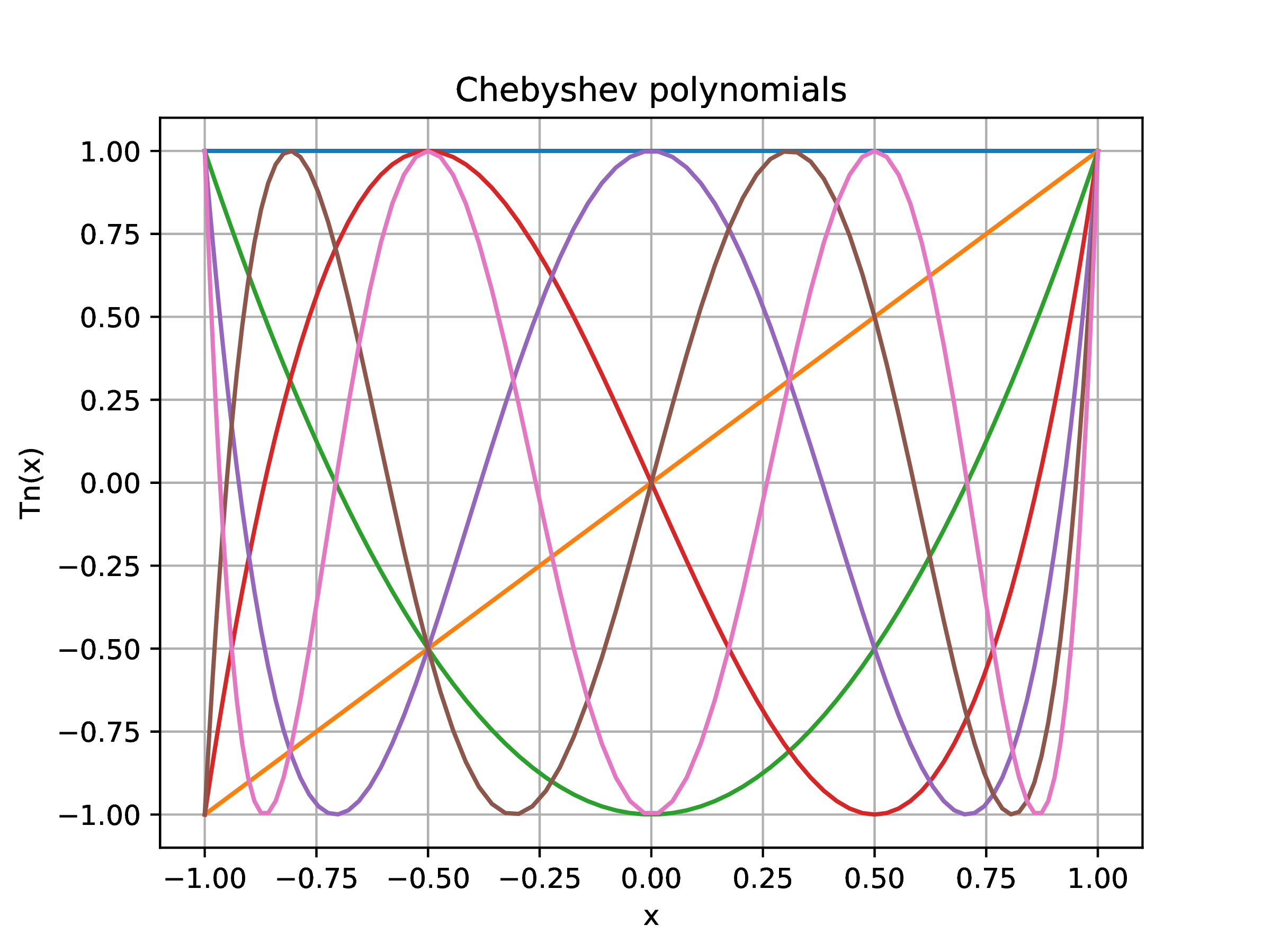
i.e., finding the sample points or roots of $w (t)$ that lead to the smallest possible inf-norm of $w (t)$ . Plots of the Lagrange basis (L18, Fig. 2), or Legendre basis, suggest study of basis functions that have distinct roots in the interval $[- 1, 1]$ and attain the same maximum. The trigonometric functions satisfy these criteria, and can be used to construct the Chebyshev family of polynomials through

T_{n} (x) = \cos [n \cos^{- 1} x] = \cos (n θ), \cos θ = x, θ = \cos^{- 1} x .

The trigonometric identity

\cos [(n + 1) θ] + \cos [(n - 1) θ] = 2 \cos θ \cos (n θ)

leads to a recurrence relation for the Chebyshev polynomials

T_{n + 1} (x) = 2 x T_{n} (x) - T_{n - 1} (x), T_{0} (x) = 1, T_{1} (x) = x .

The definition in terms of the cosine function easily leads to the roots, $T_{n} (x_{i}) = 0$ ,

\cos [n θ] = 0 \Rightarrow n θ_{i} = (2 i - 1) \frac{π}{2} \Rightarrow θ_{i} = \frac{2 i - 1}{2 n} π \Rightarrow x_{i} = \cos [\frac{2 i - 1}{2 n} π], i = 1, \dots, n,

and extrema $x_{j}$ , $T_{n} (x_{j}) = {(- 1)}^{j}$

\cos [n θ] = \pm 1 \Rightarrow n θ_{j} = j π \Rightarrow x_{j} = \cos [\frac{j π}{n}], j = 0, 1, \dots, n .

The Chebyshev polynomials are not themselves monic, but can readily be rescaled through

P_{n} (x) = 2^{1 - n} T_{n} (x), n > 0, P_{0} (x) = 1 .

Since $| T_{n} (x) | = | \cos (n θ) |$ , the above suggests that the monic polynomials $P_{n}$ have ${|| P_{n} ||}_{\infty} = 2^{1 - n}$ , small for large $n$ , and indeed the smallest possible monic polynomials in the inf-norm defined on $[- 1, 1]$ .

Theorem. The monic polynomial $p : [- 1, 1] \to ℝ$ has a inf-norm lower bound

${|| p ||}_{\infty} = {max}_{- 1 ⩽ t ⩽ 1} | p (t) | ⩾ 2^{1 - n} .$

Proof. By contradiction, assume the monic polynomial $p : [- 1, 1] \to ℝ$ has ${|| q ||}_{\infty} < 2^{1 - n}$ . Construct a comparison with the Chebyshev polynomials by evaluating $p$ at the extrema $x_{j} = \cos (j π / n)$ ,

${(- 1)}^{j} p (x_{j}) ⩽ | p (x_{j}) | < 2^{1 - n} = {(- 1)}^{j} P_{n} (x_{j}) = {(- 1)}^{j} 2^{1 - n} T_{n} (x_{j}) .$

Since the above states ${(- 1)}^{j} p (x_{j}) < {(- 1)}^{j} P_{n} (x_{j})$ deduce

${(- 1)}^{j} [p (x_{j}) - P_{n} (x_{j})] < 0, for j = 0, 1, \dots, n$ (2)

However, $p, P_{n}$ both monic implies that $p (x_{j}) - P_{n} (x_{j})$ is a polynomial of degree $n - 1$ that would change signs $n + 1$ times to satisfy (2), and thus have $n$ roots contradicting the fundamental theorem of algebra. $□$

$\circ$

Figure 2. First $n = 6$ Chebyshev polynomials

1.2.Best polynomial approximant

Based on the above the optimal choice of $n$ sample points is given by the roots

x_{i} = \cos [\frac{2 i - 1}{2 n} π], i = 1, \dots, n,

of the Chebyshev polynomial of $n^{th}$ degree $T_{n} (x)$ , in which case the interpolation error has the bound

| f (t) - p (t) | = | \frac{f^{(n + 1)} (ξ_{t})}{(n + 1)!} \prod_{i = 0}^{n} (t - x_{i}) | ⩽ \frac{| f^{(n + 1)} (ξ_{t}) |}{(n + 1)! 2^{n}} ⩽ \frac{{|| f^{(n + 1)} ||}_{\infty}}{(n + 1)! 2^{n}} .