MATH661 Scientific Computing I

MATH661
Scientific Computing I

Summary. An introduction to scientific computing theory and practice covering approximation of numbers, real functions, functionals, and operators. A presentation of classical numerical methods topics, but with a focus on how key unifying ideas naturally lead from Newtonian interpolation to deep neural networks. A literate programming and reproducible computation approach is utilized using the Julia language within live TeXmacs documents that allows simultaneous presentation of theory and implementation, as well as reproducible computational experiments, trying to adhere as much as possible to the adage:

“Beauty is truth, truth beauty, – that is all

Ye know on earth, and all ye need to know.”

John Keats, Ode on a Grecian Urn.

Course syllabus

Times	MoWe 10:10AM-11:25PM, Phillips 228
Office hours	MoWe 2:00PM-3:30PM, Tu 12:00-1:30PM Chapman 451, and by email appointment
Instructor	Sorin Mitran
Assistant	Emma Crawford (Office hours: We 9:00-10:00AM, Fr 11:30AM-12:30PM)
Jump to	Tracks: 2.2 Lessons: 3.2Homework: 3.3Software: 4.2Live documents: 4.5

(The instructor reserves the right to make changes to the syllabus. Any changes will be announced as early as possible.)

1Introduction

1.1Historical overview

Scientific computing encompasses a vast range of techniques and applications ranging from discrete computations on graphs describing social networks to stochastic molecular dynamics of protein folding. Mathematical topics that arise range from group theory and use of the Chinese Remainder Theorem to construct factorizations, to Gröbner bases to solve polynomial systems, or combining optimization theory with analysis to solve non-linear systems through a quasi-Newton method (Fig. 1).

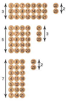
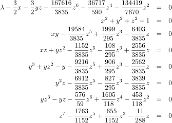
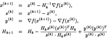
Figure 1. Left: Schematic of Chinese Remainder Theorem. Center: Gröbner basis transformation of the system $3 x^{2} + 2 yz - 2 x λ = 0$ , $2 x z - 2 y λ = 0$ , $2 xy - 2 z - 2 z λ = 0$ , $x^{2} + y^{2} + z^{2} = 1$ is actually easier to solve than the initial formulation since the last equation is only in $z$ . Right: Broyden-Fletcher-Goldfarb-Shanno algorithm to solve an optimization problem by including curvature information into a gradient descent procedure.

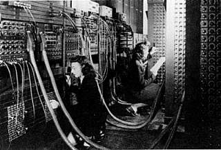
A comparably large toolkit of software applications has been developed since the first general purpose digital computer (ENIAC – Electronic Numerical Integrator and Computer) capable of about 500 FLOPS (floating point operations per second) was introduced. ENIAC was initially “programmed” by physically linking certain wires between functional units according to a flow-chart Fig. 2, a time-consuming and tedious process that was soon replaced by “coding”, the practice of specifying a sequence of logic operations to control the machine, an idea that predates ENIAC, and introduced through the assembly language of the Mark I computer input to the machine through a punched paper tape Fig. 2. This approach was still being used when your current instructor was in high school in the 1970's working on a electromechanical teleprinter, though the programming language had fortunately evolved to the more palatable BASIC language.

Figure 2. Left: Programming ENIAC by connecting wires to different functional units. Center: Flowchart guiding the wire connections. Left: Part of a punched paper tape program.

1.2Course goals

It is apparent that a single course can only provide an introduction to the myriad developments within scientific computing from the past eight decades. The main goals of this course is to explore how a few key ideas can be applied to representative problems encountered in scientific computation.

1.2.1Mathematics

There are just four mathematics ideas that are considered in this course:

Approximation: The notion of replacing some complicated mathematical object by one that is simpler to compute. In succession, the course presents the approximation of numbers, functions, and operators. The main focus is on numerical approximation, but computational analytical approximation is also presented.
Linear combination: An approach to constructing complex objects by scaling and addition of simpler objects. Note the link to approximation, in that “simpler to compute” is interpreted as scaling and addition.
Nonlinear combination: An approach to constructing complex objects by function composition, successive nonlinear transformation of simpler objects.
Limits: An approach to constructing complex objects by a sequence of approximations.

The above ideas have the character of a leitmotif in a Wagner opera: a salient feature that constantly makes its appearance throughout a work. Irrespective of the particular field of scientific computing you choose to pursue, the above ideas obstinately recur.

1.2.2Computing

Comparable simplicity is encountered in computational ideas. Even though human passion can lead to “programming language wars”, key computational concepts are few in number:

Memory management

Transfer and organization of data on a computer.

Repetition

Multiple execution of a task. Two repetition types are encountered:

Iteration: A portion of code that is repeatedly executed, typically within a loop.
Recursion: A portion of code organized as a function that calls itself.

We shall present the close correspondence between the computer science concepts of iteration and recursion to the mathematical concepts of linear and nonlinear combination, respectively.

Condition testing

Carrying out decisions based on data.

The above basic concepts have been embodied into dozens of computer languages (e.g., FORTRAN, LISP, BASIC, Pascal, ALGOL, Ada, C, C++, MATLAB, Perl, Python), with useful features from each often appearing in subsequent revisions of others (e.g., Fortran 2018 contains many features from C++ and MATLAB). In practice, a sound understanding of one language is sufficient to quickly pick up another.

This course adopts the Julia programming language, a general-purpose language that incorporates many prior ideas found useful for scientific computing.

1.2.3Scholarship

Relevance of computational approaches to science requires adoption of the scientific method of verification of the predictions resulting from conjectures (or hypotheses or theories). For scientific computing, the conjectures are the mathematical approach and implementation into a program executed by a computer. Predictions are obtained from program execution and verified by comparison to known results or experiments. Such computational predictions should be reproducible.

A key part of the scientific method is documentation of an investigation, clearly citing sources, approaches, hypotheses, and results. An important goal of this course is to instill this practice of scholarship into all aspects of scientific computing. As the case of general-purpose languages, several specialized programming languages have been developed for this purpose (TeX, LaTeX, Markdown), some with an explicit focus on documenting theoretical approach and computer implementation simultaneously (Web), a practice known as literate programming.

This graduate course utilizes a literate programming approach based upon the TeXmacs platform in conjunction with Zotero reference management. While the focus of undergraduate education is to accumulate knowledge and optionally be exposed to research, that of graduate education is to acquire the skill set needed to carry out new original research. To aid in this transition, course tasks are organized as steps in the production of a research paper. Supplementing the presentation of course topics in TeXmacs, sample documentation and Julia implementations are also provided in the Pluto environment.

1.3Course outcomes

Upon successful course completion students will be:

able to recognize particular types of approximation;
proficient in the basic operations of numerical linear algebra;
able to determine the computational complexity of an algorithm;
capable of recognizing mathematical problems that are inherently difficult to compute (e.g., “ill-conditioned”), and estimating the error arising from numerical approximation;
exposed to computational analytical approximations, and capable of comparing numerical and analytical approximations to verify algorithm performance;
introduced to both traditional additive approximations based upon linear combination and the burgeoning field of approximations based upon function composition inspired by brain functionality (neural networks).

2Course information

2.1Honor code

Unless explicitly stated otherwise, all work is individual. You may discuss various approaches to homework problems with students, instructors, but must draft your answers by yourself. All external sources consulted must be acknowledged and cited. Students implicitly accept this honor code by submission of any work for grading.

2.2Course policies

Class attendance is expected and essential for understanding of course topics. There is no need to inform instructor of planned absences. Office hour attendance is recorded and required at a minimum of one half-hour every two weeks. Self-organize into teams of two or three students and prepare questions prior to office hours. Be prepared to be quizzed on definitions during office hours. Come prepared with: notes, laptops, well-formulated questions. Students not prepared for office hours will be invited to come at a later date.

Course grade is based upon accumulation of credit points (0-100). There is no “grading on a curve”. Extra credit opportunities are offered for an additional 12 grade points, to allow for missed homework or tests.

Homework is to be submitted in typeset form (TeXmacs preferred, Pluto notebook accepted) electronically through Canvas. Handwritten homework is not accepted. The assignment deadlines are strictly enforced. Late homework is accepted only in the case of University approved class absences. E-mail messages requesting acceptance of late homework due to any other circumstance are deleted without review or response. Students are advised to prepare and submit homework well in advance of the Canvas deadline to allow for unforseen difficulties. Suspension of classes due to campus-wide events (weather, pandemic, etc.) will lead to modification of due dates or elimination of specific assignments for the entire class.

Two different tracks are offered for users and developers of scientific computation. The same theory is covered, but assignments differ between the two tracks. Both tracks are presented at the graduate level of study.

Scientific computation users. Students interested in applying existing computational techniques. Typically, most undergraduates and many non-mathematics graduates are within this group. The emphasis of the coursework is on understanding theoretical approaches and practical aspects of computing. Coursework requires only material presented in class notes.
Scientific computation developers. Students interested in extending existing computational techniques or devising new approaches. Mathematics graduate students must follow this track. Other students expecting to apply computational methods during their careers should also follow this track. This track is also available on an assignment by assignment basis to any student wishing to explore development of advanced computational methods. The emphasis of the coursework is theoretical analysis, novel algorithm formulation, and carrying out algorithm validation. Comparison of course material to alternative sources is required.

Accessibility resources and services. The University of North Carolina at Chapel Hill facilitates the implementation of reasonable accommodations, including resources and services, for students with disabilities, chronic medical conditions, a temporary disability or pregnancy complications resulting in barriers to fully accessing University courses, programs and activities.

Accommodations are determined through the Office of Accessibility Resources and Service (ARS) for individuals with documented qualifying disabilities in accordance with applicable state and federal laws. See the ARS Website for contact information: https://ars.unc.edu or email ars@unc.edu.

Counseling and psychological services (CAPS). CAPS is strongly committed to addressing the mental health needs of a diverse student body through timely access to consultation and connection to clinically appropriate services, whether for short or long-term needs. Go to their website: https://caps.unc.edu/ or visit their facilities on the third floor of the Campus Health Services building for a walk-in evaluation to learn more.

Title IX resources. Any student who is impacted by discrimination, harassment, interpersonal (relationship) violence, sexual violence, sexual exploitation, or stalking is encouraged to seek resources on campus or in the community. Reports can be made online to the EOC at https://eoc.unc.edu/report-an-incident/. Please contact the University's Title IX Coordinator (Elizabeth Hall, interim – titleixcoordinator@unc.edu), Report and Response Coordinators in the Equal Opportunity and Compliance Office (reportandresponse@unc.edu), Counseling and Psychological Services (confidential), or the Gender Violence Services Coordinators (gvsc@unc.edu; confidential) to discuss your specific needs. Additional resources are available at safe.unc.edu.

2.3Grading

Coursework involves multiple activities, differentiated between user and developer tracks.

Homework aids assimilation of basic course concepts through small-scale applications:

10 assignments $\times$ 4 points = 40 points.

Eleven assignments are given allowing students to miss one homework due to personal reasons or to use as extra credit. HW00 is meant to familiarize students with the homework drafting process and expectations, and though not graded is returned with comments that must be respected in future assignment submissions.
Projects explore medium-scale applications and scholarly practices:

2 projects $\times$ 8 points = 16 points.
Office hour participation: 8 visits $\times$ 0.5 point = 4 points.
Midterm examination 1 (in-class, 60 minutes) in Week 6 on linear algebra: 10 points.
Midterm examination 2 (in-class, 60 minutes) in Week 10 on real function approximation: 10 points.
Final examination covering all course material scheduled at 8:00AM on Th, Dec. 14, 2023: 20 points.
Extra credit on supplementary topics: 2 topics $\times$ 4 points = 8 points.
All coursework is graded at the graduate level. Undergraduate students are allocated an initial 20 course points to reward participation in an advanced course.

Mapping of point scores to letter grades

Grade	Points	Grade	Points	Grade	Points	Grade	Points
H++, A+	101-112	H-, B+	86-90	P-, C+	71-75	L-, D+	56-60
H+, A	96-100	P+, B	81-85	L+, C	66-70	L-, D	50-55
H, A-	91-95	P, B-	76-80	L, C-	61-65	F	0-49

A passing score can be obtained solely through homework, projects and office hour participation (60 points, L-/D+ grade). Undergraduate students who participate in office hours and correctly complete homework and projects attain 80 points (B- grade), with additional points available from examinations and extra credit. Latin honors are used for A+, H+, H++ grades, i.e., H++ (112 points) is entered as H with a transcript annotation of summa cum laude, at instructor's discretion.

3Lesson plan

3.1Course modules

Though unitary in nature, the course is organized in distinct modules that may be useful for auditors from diverse backgrounds not interested in taking the full course.

Module	Topics
Number approximation	Computational representations of $ℕ, ℤ, ℚ, ℝ, ℂ$
Numerical linear algebra	Introduction to approximation by linear combination.
Real function approximation	Approximation of functions $f : ℝ \to ℝ$
Linear operator approximation	Approximation of linear functions defined on a vector space $𝒰$ , i.e., scalar-valued linear functionals $f : 𝒰 \to ℝ$ , and vector-valued linear operators $f : 𝒰 \to 𝒱$ .
Nonlinear operator approximation	Approximation of non-linear functionals and operators.

3.2Course topics, test dates, and notes

Midterm dates are indicated in bold red.

Lesson Schedule

Week	Notes	Exercises	Date	Topic
01	L01 L02 L03	E01 E02	08/21 08/23	Floating point arithmetic. Approximating sequences. Order of convergence. Finite difference approximation of derivative and catastrophic loss of precision. Condition number.
02	L04 L05 L06	E03	08/28	Linear combinations. Vector and matrix norms. Linear functionals and mappings. Vector spaces and subspaces. Bases. Dimension. Orthogonal matrices. Matrix subspaces.
03	L07 L08 L09		09/06	Bases. Dimension. Orthogonal matrices. Matrix subspaces. Fundamental theorem of linear algebra. Rank-nullity.
04	L10 L11 L12	E04	09/11 09/13	Singular value decomposition theorem & proof. Karhunen-Loève. Rank-1 expansions. Operator approximation. Linear statement of applied mathematics problems: coordinate changes (linear systems), reduced-order models (least squares), operator invariants (eigenproblems). SVD solutions. Pseudo-inverse.
05	L13 L14 L15		09/18 09/20	$Q R$ least-squares solution. Additional operator representations: $Q R$ , $L U$ , $L L^{}$ , $Q T Q^{}$ . Computational complexity. Projection: Householder, Givens. Eigenvalue algorithms, Rayleigh iteration.
06			09/27	Midterm examination 1 on linear algebra topics.
07	L18 L19		10/02 10/04	Approximation in the monomial basis. Interpolation. Newton, Lagrange forms. Taylor series. Polynomial interpolation error.
08	L20 L21		10/09 10/11	Hermite interpolation. Splines. $B$ -spline basis. Finite elements.
09	L22 L23		10/16 10/18	Approximation in spectral bases. Fourier, Wavelet approximations. $L_{1}, L_{2}, L_{\infty}$ approximants. Minimax.
10	L24		10/23 10/25	Midterm examination 2 on real function approximation.
11	L25 L26	E07	10/30 11/01	Linear operator approximation 1: quadrature ( $\int d x^{n}$ ). Newton-Cotes. Moments. Gauss quadrature. Convergence. Romberg. Linear operator approximation 2: differentiation ( $d^{n} / d x^{n}, \nabla, \nabla^{2}$ ).
12	L27 L28		11/06 11/08	Linear ODE ( $\sum_{k} a_{k} d / d x^{k}$ ). Convergence. Stability
13	L29 L30		11/13 11/15	Non-linear operator approximation 1: $f : ℝ \to ℝ, f (x) = 0,$ 0,1,2-degree approximants (secant, Newton, Steffensen, Halley, Householder). Convergence, fixed points.
14	L31 L32		11/20	Non-linear operator approximation 2: $f : ℝ^{n} \to ℝ, f (x) = 0$ . 0,1,2-degree approximants. Convexity, steepest descent. Stochastic steepest descent.
15	L33 L34		11/27 11/29	Non-linear operator approximation 3: $F : ℝ^{n} \to ℝ^{n}, F (x) = 0$ . Quasi-Newton methods.
16	L35 L36		12/04 12/06	Non-linear combinations. Neural networks. Neural network approximation of real scalar functions, real functionals, real vector functions. Neural network approximation of operators.

3.3Homework and Projects

Nr.	Topic	Issue Date	Due Date	Problems	Solution
HW00	Number approximation	08/23	09/06	H00	S00
HW01	Numerical linear algebra
HW02		09/06	09/13	H02	S02
HW03		09/13	09/20	H03	S03
HW04		09/20	09/27	H04	S04
P01		10/02	10/16,11/20	P01
HW05		10/04	10/11	H05	S05
HW06	Real function approximation	10/11	10/18	H06	S06
HW07		10/16	10/23	H07	S07
EC		10/25	11/08	EC
HW08	Linear operator approximation	10/25	11/06	H08	S08
HW09		11/13	11/20	H09	S09
P02		11/15	11/27	P02
HW10	Nonlinear operator approximation	11/27	12/06	H10	S10
HW11		11/29	12/06	H11	S11

3.4Test preparation and solutions

	Midterm 1	Midterm 2	Final
Questions	M1	M2
Solutions	M1Sol	M2Sol

3.5Extra credit topics

For each of the topics below:

read the relevant class notes or indicated textbook presentation

look up and read original sources

try a small sample computation

present influence of work in the field by following citations of original sources

Nr.	Issue Date	Due Date	Topic
01	09/27	10/23	Linear model reduction
02	10/23	12/04	Fractional derivative approximation

3.6Bibliography

Course textbook: Scientific Computation by S. Mitran.

Perusal of the following texts is highly recommended for all, and is required for Track 2 students who can expect to be quizzed on topics from these texts during office hour visits.

Numerical Linear Algebra, by L.N. Trefethen and D. Bau.

Matrix Computations, by G.H. Golub and C.F. Van Loan

Applied Numerical Linear Algebra, by J.W. Demmel

Matrix Iterative Analysis, by R.S. Varga

Methods of Mathematical Physics, by R. Courant and D. Hilbert

Methods of Theoretical Physics, by P.M. Morse and H. Feshbach

Mathematics for the Physical Sciences, by L. Schwartz

Computational Functional Analysis, by R. Moore

4Computational resources

4.1Hardware

Students are required to have a computer, preferably a laptop, that conforms to CCI minimal standards. Current computers use either a CISC (complex instruction set computer) or RISC (reduced instruction set computer) architecture. A recommended laptop based on the CISC Intel x86-64 architecture would be equipped with a 6-core processor, 4 GB NVIDIA GPU, 16GB RAM, 512 GB SSD or better. A recommended laptop based on the Apple arm64 RISC architecture would be equipped with an 8-core processor, 16GB unified RAM, 512 GB SSD or better. The course will explore algorithm parallelism both on multi-core CPUs and on GPUs, and algorithm verification will often require consideration of larger problems.

4.2Software

Modern software systems allow efficient, productive formulation and solution of mathematical models. A key goal of the course is to familiarize students with these capabilities and acquire the practical skills needed for scientific computing. Three software approaches are possible:

Preconfigured virtual machine

This is the preferred and fully supported option. On machines with the x86-64 architecture, install the SciComp@UNC environment in which tools required for modern scientific computation have been preconfigured for immediate use. Follow instructions at SciComp@UNC to install on a laptop with at least 24GB free disk space and 8GB RAM.

Individual software package installation

For students comfortable in system administration. Limited support only for arm64 architecture. On machines with either x86-64 or arm64 architecture, install the main software packages used in the course.

Windows OS.

Create a directory named C:\courses
Install TortoiseSVN
Open File Explorer and right-click to open options (“See more options” in Windows 11) for folder C:\courses. Select SVN checkout option and enter:

URL repository: svn://mitran-lab.amath.unc.edu/courses/MATH661

Checkout directory: C:\courses\MATH661

Click OK, and a copy of the course material repository is downloaded to your laptop.
Julia programming language. Choose installation directory C:\courses\julia

Modify the System variable PATH to include C:\courses\julia\bin

In Julia terminal session install the Printf, Latexify, PyPlot, LinearAlgebra, Revise packages. Add the path to the julia executable to your system PATH variable. For example, to install Latexify within a Julia session:
∴

import Pkg
∴

Pkg.add("Latexify")
TeXmacs editing platform. Choose installation directory C:\courses\texmacs
Zotero reference management system.
Open File Explorer and right-click to open options (“See more options in Windows 11”) for folder C:\courses\texmacs\plugins. Select SVN checkout option and enter:

URL repository:

svn://mitran-lab.amath.unc.edu/courses/texmacs/plugins/julia

Checkout directory: C:\courses\texmacs\plugins\julia

Mac OS.

Open the Terminal app and create a directory named ~/courses
```
cd ~; mkdir courses
```
Install SmartSVN
Open SmartSVN and select option Check out project from repository, click OK. Enter:

Repository: svn://mitran-lab.amath.unc.edu/courses/MATH661, select MATH661 directory

Local directory: ~/courses/MATH661

Click Continue, and a copy of the course material repository is downloaded to your laptop.
Julia programming language. Choose installation directory C:\courses\julia

Modify the System variable PATH to include /Applications/Julia-1.6.app/Contents/Resources/julia/bin

In Julia terminal session install the Printf, Latexify, PyPlot, LinearAlgebra packages. Add the path to the julia executable to your system PATH variable. For example, to install Latexify within a Julia session:
∴

import Pkg
∴

Pkg.add("Latexify")
TeXmacs editing platform.
Zotero reference management system.
Open SmartSVN and select option Check out project from repository, click OK. Enter:

Repository:

svn://mitran-lab.amath.unc.edu/courses/texmacs/plugins/julia

Checkout directory: /Applications/TeXmacs.app/Contents/Resources/share/TeXmacs/plugins

Students are responsible for software configuration. Help will be given through posted instructions within available time. Since the course focuses on the mathematics of scientific computing, e-mail or office hour support for this software option is not possible, and such requests will uniformly be answered by the suggestion to install the preconfigured SciComp@UNC environment.

4.3Tutorials

Software usage is introduced gradually in each class, so the first resource students should use is careful, active reading of the material posted in class. In particular, carry out small tasks until it becomes clear what the software commands accomplish. Some additional resources:

TeXmacs:

Julia:

4.4Course material repository

Course materials are stored in a repository that is accessed through the subversion utility, available on all major operating systems. The URL of the material is svn://mitran-lab.amath.unc.edu/courses/MATH661

In the SciComp@UNC virtual machine the initial checkout can be carried out through the terminal commands

cd ~/courses

make MATH661

Update the course materials before each lecture by:

cd ~/courses/MATH661

svn update

Links to course materials will also be posted to this site, but the most up-to-date version is that from the subversion repository, so carry out the svn update procedure prior to each lecture.

4.5Interactive documents

All course material is presented as TeXmacs documents with embedded interactive Julia sessions. Such documents have a .tm extension and are available through svn download from the course repository. Notes posted on the lesson plan contain translations of the live documents to .pdf formats.

Live documents allow immediate application of course topics, shown here for the simple case of a bisection method to solve the equation $f (x) = 0$ , when $f \in C [a, b]$ , and $f (a) f (b) ⩽ 0$ . The algorithm constructs sequences ${a_{n}}_{n \in ℕ}$ , ${b_{n}}_{n \in ℕ}$ that bracket the root $c$ , with the root approximation at iteration $n$ given by $c_{n} = (a_{n} + b_{n}) / 2$ to within a maximum absolute error of $δ_{n} = (b_{n} - a_{n}) / 2$ .

Algorithm - Bisection method

Input: $f, a, b, ε$

if $a > b$ then $swap (a, b)$

$fa \leftarrow f (a)$ ; $fb \leftarrow f (b)$

$δ \leftarrow b - a$

while $δ > ε$ and $fa \cdot fb ⩽ 0$

$δ \leftarrow δ / 2$ ; $c \leftarrow a + δ$ ; $fc \leftarrow f (c)$

if $fa \cdot fc ⩽ 0$

$b \leftarrow c$ ; $fb \leftarrow fc$

else

$a \leftarrow c$ ; $fa \leftarrow fc$

return $c$

Julia (1.6.1) session in GNU TeXmacs

∴	function bisect(f,a,b,ε) if (a>b) a,b=b,a end fa=f(a); fb=f(b) δ=b-a; c=(a+b)/2 while ((δ>ε) && (fafb<=0)) δ=δ/2; c=a+δ; fc=f(c) if (fafc<=0) b,fb=c,fc else a,fa=c,fc end end return c end;

∴	f(x)=x^2-2; a=1; b=2; ε=0.01;

∴	[bisect(f,a,b,ε) sqrt(2.0)]

$[\begin{array}{cc} 1.4140625 & 1.4142135623730951 \end{array}]$ (1)

∴	g(x)=x^2-3; a=1; b=2; ε=0.001;

∴	[bisect(g,a,b,ε) sqrt(3.0)]

$[\begin{array}{cc} 1.7314453125 & 1.7320508075688772 \end{array}]$ (2)

∴

Pluto has an analogous approach, but with fewer capabilities, e.g., the table organization shown above that allows immediate transcription of the pseudocode for the bisection method into Julia. More importantly, TeXmacs is an efficient medium for prototyping ideas and subsequently transforming them into formal scientific communication, i.e., research papers.