Solve the problems for your appropriate course track. Problems probe understanding of the definitions and results from the module on function approximation through linear combination. Formulate your answers clearly, cogently, and include a concise description of your approach. Each question is meant to be completely answered within ten minutes. Allowed test time is 75 minutes.

1Track 1

1. Construct the polynomial interpolant of data $𝒟=\{(-1,-6),(0,-1),(1,-2),(2,-3)\}$ in Lagrange form.

   Solution. With $𝒙={\left[\begin{array}{llll}-1& 0& 1& 2\end{array}\right]}^T$, $𝒚={\left[\begin{array}{llll}-6& -1& -2& -3\end{array}\right]}^T$, the cubic Lagrange polynomial interplant is

   ${\displaystyle p_3\left(t\right)=\sum _{k=1}^4{y}_k{\ell }_k\left(t\right),}$
   ${\displaystyle \begin{array}{ll}{\ell }_1\left(t\right)=\frac{(t-x_2)(t-x_3)(t-x_4)}{(x_1-x_2)(x_1-x_3)(x_1-x_4)}=\frac{t(t-1)(t-2)}{(-1)(-2)(-3)}& {\ell }_2\left(t\right)=\frac{(t-x_2)(t-x_3)(t-x_4)}{(x_1-x_2)(x_1-x_3)(x_1-x_4)}=\frac{(t+1)t(t-1)}{\left(1\right)(-1)(-2)}\\ {\ell }_3\left(t\right)=\frac{(t-x_1)(t-x_2)(t-x_4)}{(x_3-x_1)(x_3-x_2)(x_3-x_4)}=\frac{(t+1)t(t-2)}{\left(2\right)\left(1\right)(-1)}& {\ell }_4\left(t\right)=\frac{(t-x_1)(t-x_2)(t-x_3)}{(x_4-x_1)(x_4-x_2)(x_4-x_3)}=\frac{(t+1)t(t-1)}{\left(3\right)\left(2\right)\left(1\right)}\end{array}}$

2. Construct the Newton form of the polynomial interpolant of the above data set, presenting the table of divided differences.

   Solution. Table of divided differences

   ${\displaystyle \begin{array}{llllll}i& x_i& y_i& [y_i,y_{i-1}]& [y_i,y_{i-1},y_{i-2}]& [y_i,y_{i-1},y_{i-2},y_{i-3}]\\ 1& -1& -6& -& -& -\\ 2& 0& -1& 5& -& -\\ 3& 1& -2& -1& -3& -\\ 4& 2& -3& -1& 0& 1\end{array},}$

   leads to Newton interpolant

   ${\displaystyle p_3\left(t\right)=-6+5(t+1)-3(t+1)t+(t-1)(t+1)t.}$

   Verify: $p_3(-1)=-6,p_3\left(0\right)=-1,p_3\left(1\right)=-2,p_3\left(2\right)=-3.?$

3. Efficiently evaluate the Newton form of the polynomial interpolant determined above at $t=2$, using Horner's scheme. Present a pseudo-code algorithm.

   Solution. For known divided differences $𝒅=\left[\begin{array}{llll}{y}_0& [y_1,y_0]& ..& [y_n,..,y_1,y_0]\end{array}\right]$ on the diagonal of the table, an $𝒪\left(n\right)$ scheme is

   Algorithm

   Input: $n,t,x,d$

   $p=d_{n+1}$

   for $j=n$ downto $1$

   $p=p\cdot (t-x_j)+d_j$

   end

   return $p$

4. Replace the sampling points $x_i=-1+i$, $i=0,..,3$ in the data set $𝒟$ so as to minimize the interpolation error over the interval $[-1,2]$.

   Solution. The error is minized for the Chebyshev points, i.e., roots of $T_4\left(z\right)=0$, scaled to cover the interval $[-1,2]$ by $x\left(z\right)=\frac{3}{2}(z+1)-1$. Roots of $T_4\left(\theta \right)=\cos \left(4\theta \right)=0$ are ${\theta }_j=\frac{\pi }{4}(\frac{1}{2}+j\pi )$, for $j=0,1,2,3$, with $z_j=\cos {\theta }_j$, $x_j=\frac{3}{2}(z_j+1)-1$.

2Track 2

1. Construct the Hermite interpolant of data $𝒟=\{(x_i,y_i=f\left(x_i\right),y_i^{\text{'}}=f^{\text{'}}\left(x_i\right)),i=0,1\}=\{(-1,-6,10),(0,-1,1)\}$ in Newton form.

   Solution. The table of divided differences with repetitions

   ${\displaystyle \begin{array}{llllll}i& x_i& y_i& [y_i,y_{i-1}]& [y_i,y_{i-1},y_{i-2}]& [y_i,y_{i-1},y_{i-2},y_{i-3}]\\ 0& -1& y_0=-6& -& -& -\\ 0& -1& -6& y_0^{\text{'}}=10& -& -\\ 1& 0& y_1=-1& 5& -5& -\\ 1& 0& -1& y_1^{\text{'}}=1& -4& 1\end{array},}$

   leads to the cubic polynomial

   ${\displaystyle p_3\left(t\right)=-6+10(t+1)-5{(t+1)}^2+{(t+1)}^{2}t.}$

   Verify

   ${\displaystyle p_3(-1)=-6,p_3\left(0\right)=-6+10-5=-1,?}$ ${\displaystyle p_3^{\text{'}}\left(t\right)=10-10(t+1)+{(t+1)}^2+2(t+1)t,}$
   ${\displaystyle p_3^{\text{'}}(-1)=10,p_3^{\text{'}}\left(0\right)=10-10+1=1.?}$

2. Construct the Hermite interpolant of the above data in the Lagrange form

   ${\displaystyle p\left(t\right)=\sum _{i=0}^n[a_i\left(t\right)y_i+b_i\left(t\right)y_i^{\text{'}}],}$

   where $a_i\left(x_j\right)={\delta }_{ij}$, $a_i^{\text{'}}\left(x_j\right)=0$, $b_i^{\text{'}}\left(x_j\right)={\delta }_{ij}$, $b_i\left(x_j\right)=0$.

   Solution. Repeat the divided difference table with symbols for function, derivative values

   ${\displaystyle \begin{array}{llllll}i& x_i& y_i& [y_i,y_{i-1}]& [y_i,y_{i-1},y_{i-2}]& [y_i,y_{i-1},y_{i-2},y_{i-3}]\\ 0& -1& y_0& -& -& -\\ 0& -1& y_0& y_0^{\text{'}}& -& -\\ 1& 0& y_1& y_1-y_0& y_1-y_0-y_0^{\text{'}}& -\\ 1& 0& y_1& y_1^{\text{'}}& y_1^{\text{'}}-(y_1-y_0)& y_1^{\text{'}}-2(y_1-y_0)+y_0^{\text{'}}\end{array},}$

   giving

   ${\displaystyle p_3\left(t\right)=y_0+y_0^{\text{'}}(t+1)+(y_1-y_0-y_0^{\text{'}}){(t+1)}^2+(y_1^{\text{'}}-2(y_1-y_0)+y_0^{\text{'}}){(t+1)}^{2}t.}$

   Gather terms

   ${\displaystyle p_3\left(t\right)=[1-{(t+1)}^2+2{(t+1)}^{2}t]y_0+[{(t+1)}^2-2{(t+1)}^{2}t]y_1+[(t+1)-{(t+1)}^2+{(t+1)}^{2}t]y_0^{\text{'}}+{(t+1)}^{2}t{y}_1^{\text{'}}.}$

   Identify and verify conditions

   ${\displaystyle \begin{array}{llll}{a}_0\left(t\right)={(t+1)}^2(2t-1)+1,& a_0(-1)=1,& a_0\left(0\right)=0,& ?\\ a_0^{\text{'}}\left(t\right)=2{(t+1)}^2+2(t+1)(2t-1),& a_0^{\text{'}}(-1)=0,& a_0^{\text{'}}\left(0\right)=0,& ?\\ a_1\left(t\right)={(t+1)}^2(1-2t),& a_1(-1)=0,& a_1\left(0\right)=1,& ?\\ a_1^{\text{'}}\left(t\right)=2(t+1)(1-2t)-2{(t+1)}^2,& a_1^{\text{'}}(-1)=0,& a_1^{\text{'}}\left(0\right)=0,& ?\\ b_0\left(t\right)=t+1+(t-1){(t+1)}^2,& b_0(-1)=0,& b_0\left(0\right)=0,& ?\\ b_0^{\text{'}}\left(t\right)=1+{(t+1)}^2+2(t^2-1),& b_0^{\text{'}}(-1)=1,& b_1^{\text{'}}\left(0\right)=0,& ?\\ b_1\left(t\right)={(t+1)}^{2}t,& b_1(-1)=0,& b_1\left(0\right)=0,& ?\\ b_1^{\text{'}}\left(t\right)={(t+1)}^2+2(t+1)t,& b_1^{\text{'}}(-1)=0,& b_1^{\text{'}}\left(0\right)=1& ?\end{array}}$
   ${\displaystyle }$

3. Present a spline interpolant $S$ of data set $𝒟=\{(x_i=ih,y_i=f\left(x_i\right)),i=0,..,n\}$, $h=1/n$, where the restriction of $S$ to interval $[x_{i-1},x_i]$ is of the form

   ${\displaystyle S_i\left(t\right)=a_i+b_i{e}^t+c_i{e}^{-t}.}$

   Solution. Impose interpolation conditions in function values

   ${\displaystyle S_i\left(x_{i-1}\right)=a_i+b_i{e}^{(i-1)h}+c_i{e}^{-(i-1)h}=y_{i-1},i=1,2,..,n}$ ${\displaystyle S_i\left(x_i\right)=a_i+b_i{e}^{ih}+c_i{e}^{-ih}=y_{i-1},i=1,2,..,n.}$

   The above specify $2n$ conditions for $3n$ parameters. Impose continuity of function derivative

   ${\displaystyle S_i^{\text{'}}\left(x_i\right)=S_{i+1}^{\text{'}}\left(x_i\right)\Rightarrow b_i{e}^{ih}+c_i{e}^{-ih}=b_{i+1}{e}^{ih}+c_{i+1}{e}^{-ih},i=1,2,,n-1,}$

   for a total of $3n-1$ condition. One additional condition is required, e.g., $S_1^{\text{'}}\left(x_0\right)=S^{\text{'}}\left(x_1\right)$ or $S_n^{\text{'}}\left(x_n\right)=S_n^{\text{'}}\left(x_{n-1}\right)$ (derivative extrapolation).

4. Find the best inf-norm approximants of $f:[0,\pi /2]\to ℝ$, $f\left(t\right)=\cos t$ by polynomials of degree $n=0,1,2$.

   Solution. For $n=0$, $f\left(t\right)\cong p_0\left(t\right)=a$, $f\left(t\right)-p_0\left(t\right)$ is monotone on $[0,\pi /2]$ and error extrema $e_0\left(t\right)=f\left(t\right)-p_0\left(t\right)$ are obtained at endpoints of compact interval $[0,\pi /2]$. By equioscillation theorem, $1-a=a\Rightarrow a=1/2$.

   

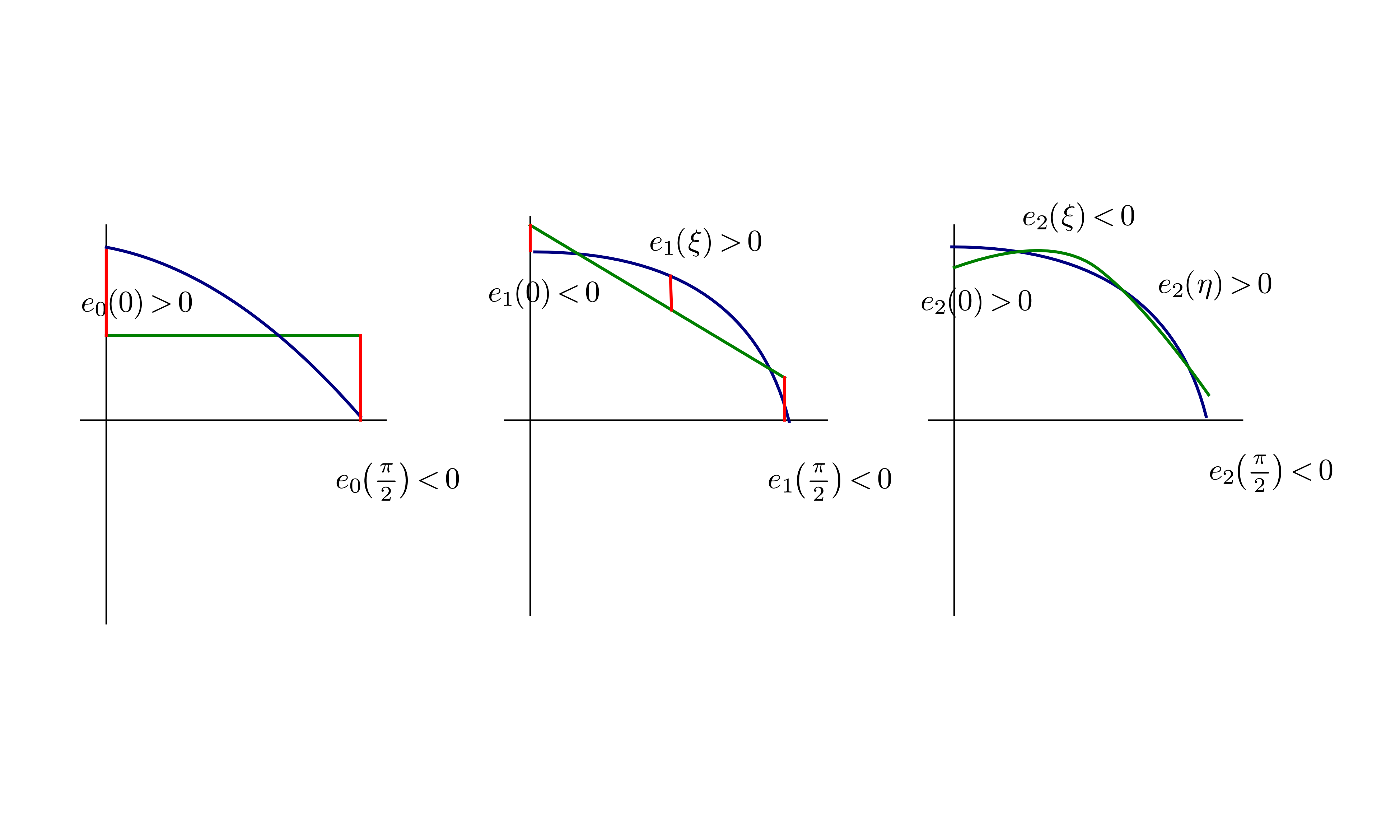
   For $n=1$, error $e_1\left(t\right)=\cos t-at-b$ has two extrema $1-b$,$a\pi /2+b$ at endpoints and a local extremum where $e_1^{\text{'}}\left(\xi \right)=0\Rightarrow -\sin \xi =a\Rightarrow \xi =-\arcsin a$. Impose equioscillation conditions

   ${\displaystyle b-1=a\pi /2+b=\cos \xi -a\xi -b,}$

   giving $a=-2/\pi$ and $b=\frac{1}{2}[\sqrt{1-a^2}+a\arcsin a+1]$.

   For $n=2$, error $e_2\left(t\right)=\cos t-a{t}^2-bt-c$ has two extrema $1-c$,$-a{(\pi /2)}^2-b(\pi /2)-c$ at endpoints. The local extremum condition $e^{\text{'}}\left(t\right)=-\sin t-2at-b=0$ is satisfied at two roots $\xi ,\eta$ (consider best approximant of $\sin t$ by a polynomial of degree 1 with similar solutions as that for $\cos t$). Apply equioscillation theorem

   ${\displaystyle 1-c=a{(\pi /2)}^2+b(\pi /2)+c=-(\cos \xi -a{\xi }^2-b\xi -c)=\cos \eta -a{\eta }^2-b\eta -c.}$

   The above requires a numerical solution.