|
|||
|
Posted: 10/02/23
Due: 10/16/21, 11:55PM (first draft, comments will be returned, revision due on 10/30)
This project presents a typical medium-size problem involving the concepts from approximation using linear combinations: transformation of coordinates, least squares, different types of basis sets.
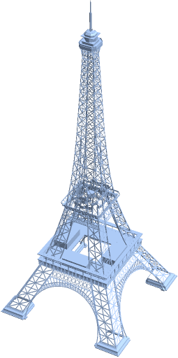
Many systems consist of point interactions. The iconic Eiffel Tower can be modeled through the trusses linking two points with coordinates . The unit vector along direction from point to point is
Suppose that structure deformation changes the coordinates to , . The most important structural response is a force exerted on point that can be approximated as
in appropriate physical units. An opposite force acts on point by principle of action and reaction. Note the projector along the truss direction , allowing computation of nodal forces as
Adding forces on a point from all trusses leads to the linear relation
| (1) |
with the forces and displacements, the stiffness matrix, the number of dimensions, the number of points, and , the number of degrees of freedom of the structure. This is a simple example of a finite element method. The vectors contain the forces, displacements at all nodes, e.g.,
with each . Assembly of the stiffness matrix is carried out by adding contributions from each truss
Such point interactions arise in molecular or social interactions, cellular motility, and economic exchange much in the same form (1). The techniques in this homework are thus equally applicable to physical chemistry, sociology, biology or business management.
Problem setup is carried through the following steps.
Add required Julia packages.
Load the data.
The following are typical instructions: open a file, load data, close the file.
∴ |
ddir = homedir()*"/courses/MATH661/data/EiffelTower"; |
∴ |
using MAT |
∴ |
Load the model point coordinates, display the first 3 node coordinates
∴ |
dfile = matopen(ddir*"/EiffelPoints.mat"); |
∴ |
X=read(dfile,"Expression1"); |
∴ |
close(dfile); |
∴ |
NX,ndims=size(X); |
∴ |
X[1:3,:] |
(2)
∴ |
Load the model edges (links between the nodes) as floating point numbers (Matlab .mat file format)
∴ |
dfile = matopen(ddir*"/EiffelLines.mat"); |
∴ |
flL=read(dfile,"Expression1"); |
∴ |
close(dfile); |
∴ |
Display model size
∴ |
NL,nseg=size(flL); [NX ndims NL nseg] |
(3)
∴ |
The model contains nodes (points) each with coordinates and edges (links) between node pairs. Transform the links to integers and display the first 4 edges.
∴ |
L=zeros(Int64,NL,nseg); |
∴ |
for l=1:NL L[l,:] = floor.(Int64,flL[l,:]) end |
∴ |
L[1:4,:] |
(4)
∴ |
The above states the first edge is from node to node .
Define the system matrix .
The data contains points in , , and line segments defined by 2 endpoints. The total number of degrees of freedom is . Of the possible linkages between points in the structure, only are present.
∴ |
m=3*NX; [NX NX^2 NL m m^2] |
(5)
∴ |
The matrix can be formed by loops over the trusses as shown in the algorithm below.
Algorithm assembly for to ; ; ; ; for to for to
end end end |
|
Define a function to carry out the assembly process in dimensions that returns a full matrix .
∴ |
function assembleK(d,L,X)
  NL = size(L)[1]; n=maximum(L); m=d*n; K=zeros(m,m)
  for k=1:NL
    i=L[k,1]; j=L[k,2]
    l=X[j,1:d]-X[i,1:d]; l=l/norm(l)
    p=d*(i-1); q=d*(j-1); P=l*l'
    for id=1:d
      for jd=1:d
        K[p+id,p+jd] = K[p+id,p+jd] - P[id,jd]
        K[p+id,q+jd] = K[p+id,q+jd] + P[id,jd]
        K[q+id,p+jd] = K[q+id,p+jd] + P[id,jd]
        K[q+id,q+jd] = K[q+id,q+jd] - P[id,jd]
      end
    end
  end
  return K
end; |
∴ |
∴ |
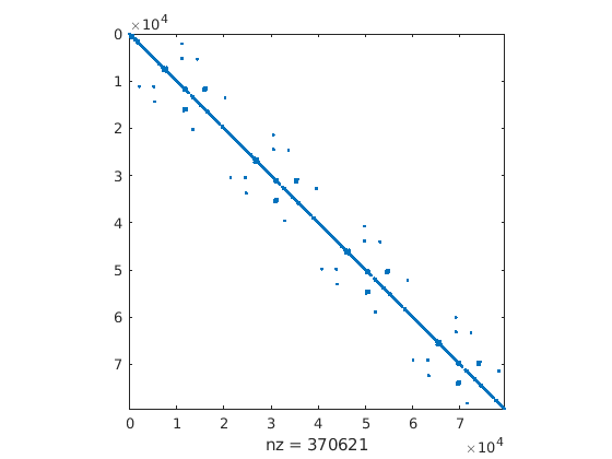
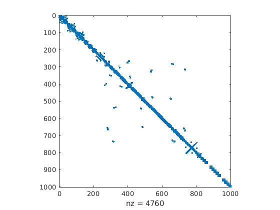
The above has been precomputed for the Eiffel Tower model. It is wasteful, and often impossible due to memory constraints, to store the entire matrix of possible couplings between points () since most of the matrix would consist of zero entries. Rather, only the nonzero elements corresponding to the linked nodes are stored through what is known as a sparse matrix. There are various techniques to store sparse matrices, one of which is the coordinate format defined by a vector of row indices , a vector of column indices and a vector of values such that the element of the matrix is
The following instructions load the sparse representation of .
∴ |
dfile = matopen(ddir*"/KCOO.mat"); |
∴ |
flrows=read(dfile,"rows"); |
∴ |
flcols=read(dfile,"cols"); |
∴ |
vals=read(dfile,"vals"); |
∴ |
close(dfile); |
∴ |
nz=size(flrows)[1] |
∴ |
rows=zeros(Int64,nz,1); cols=zeros(Int64,nz,1); |
∴ |
for l=1:nz rows[l] = floor(Int64,flrows[l]) cols[l] = floor(Int64,flcols[l]) end |
∴ |
[minimum(rows) maximum(rows) minimum(cols) maximum(cols)] |
(6)
∴ |
∴ |
using SparseArrays |
∴ |
K=sparse(rows[:,1],cols[:,1],vals[:,1]); |
∴ |
size(K) |
(7)
∴ |
K[5,6] |
∴ |
[rows[56] cols[56] vals[56]] |
(8)
∴ |
K[22,14] |
∴ |
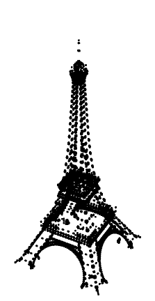
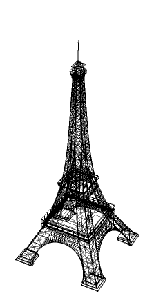
Draw the deformed structure in figure , given node coordinates , displacements , , skipping nodes (to reduce drawing time).
Draw the deformed structure in figure , given node coordinates , displacements , , skipping nodes.
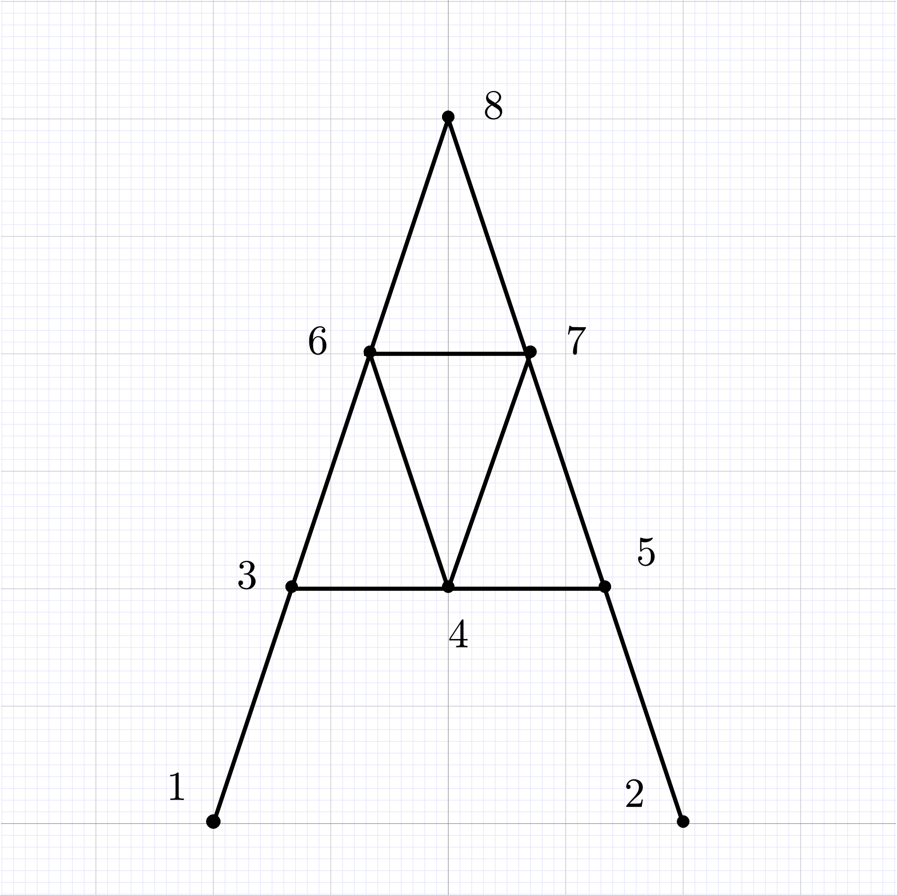
The full Eiffel Tower model is quite complex. It is convenient to build familiarity with modeling binary interactions using the much simpler two-dimensional () 8-node model shown in Fig. 3
When structures are attached to their environment, boundary conditions have to be enforced in the linear system . A common technique is set the diagonal element of for the node subjected to boundary conditions to a large value such that it effectively decouples from the system, and set where is the desired boundary value.
Construct (node coordinates, edges, stiffness matrix) for the “A” model. For this small model a sparse representation of is not required.
Start your investigation of the system by finding the largest singular values and eigenvalues of . Plot the first singular modes and eigenmodes.
Find the linear combination of the first singular modes that best approximates a force on the structure by solving the problem
Randomly choose . This is the response of the structure to wind along direction . Form and solve the analogous problem for the “A” model first.
Find the linear combination of the first eigenmodes modes that best approximates a force on the structures. Form and solve the analogous problem for the “A” model first.
Replace singular modes or eigenmodes by orthogonal , with (known as Krylov modes). Find the linear combination of the first 10 Krylov modes that best approximates a force on the structure. Form and solve the analogous problem for the “A” model first.
Carry out a bibliographic search for review papers on reduced order modeling. Choose a paper you find appealing and draft a two-paragraph summary. Compare the approach you find in the literature to problems 3 to 5 above.