MATH661 Project 2
Large system
factorization and model reduction:
Time-dependent
case |
|
Posted: 11/15/23
Due: 10/27/23, 11:55PM
This project extends the study of static binary interactions from
Project 1 to time-dependent interactions.
1Introduction
1.1Modeling binary interaction in science and
engineering
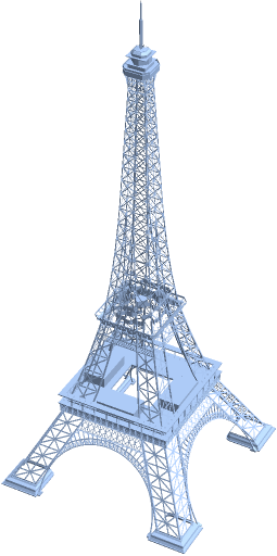
Many systems consist of point interactions. The iconic Eiffel Tower can
be modeled through the trusses linking two points with coordinates .
The unit vector along direction from point
to point is
Suppose that structure deformation changes the coordinates to ,
.
The most important structural response is a force
exerted on point that can be approximated
as
in appropriate physical units. An opposite force
acts on point by principle of action and
reaction. Note the projector along the truss direction ,
allowing computation of nodal forces as
Adding forces on a point from all trusses leads to the linear relation
with
the forces and displacements,
the stiffness matrix,
the number of dimensions, the number of
points, and ,
the number of degrees of freedom of the structure. This is a simple
example of a finite element method. The vectors
contain the forces, displacements at all nodes, e.g.,
with each .
Assembly of the stiffness matrix is
carried out by adding contributions from each truss
Such point interactions arise in molecular or social interactions,
cellular motility, and economic exchange much in the same form (1). The
techniques in this homework are thus equally applicable to physical
chemistry, sociology, biology or business management.
|
|
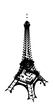
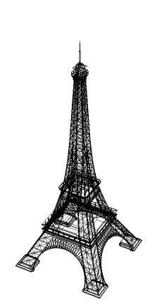
Figure 1. (Left) Eiffel Tower model. (Center)
Model nodes. (Right) Model edges.
|
1.2Problem data
Problem setup is carried through the following steps.
Add required Julia packages.
The Eiffel Tower data is available as Matlab format (.mat) files, so
we'll need a package to load the data.
∴ |
import Pkg; Pkg.add("MAT") |
Resolving package versions…
No Changes to
‘~/.julia/environments/v1.9/Project.toml‘
No Changes to
‘~/.julia/environments/v1.9/Manifest.toml‘
Load the data.
The following are typical instructions: open a file, load data,
close the file.
∴ |
ddir = homedir()*"/courses/MATH661/data/EiffelTower"; |
Load the model point coordinates, display the first 3 node
coordinates
∴ |
dfile = matopen(ddir*"/EiffelPoints.mat"); |
∴ |
X=read(dfile,"Expression1"); |
|
(2) |
Load the model edges (links between the nodes) as floating point
numbers (Matlab .mat file format)
∴ |
dfile = matopen(ddir*"/EiffelLines.mat"); |
∴ |
flL=read(dfile,"Expression1"); |
Display model size
∴ |
NL,nseg=size(flL); [NX ndims NL nseg] |
The model contains
nodes (points) each with
coordinates and
edges (links) between node pairs. Transform the links to integers
and display the first 4 edges.
∴ |
L=zeros(Int64,NL,nseg); |
∴ |
for l=1:NL
  L[l,:] = floor.(Int64,flL[l,:])
end |
|
(4) |
The above states the first edge is from node
to node .
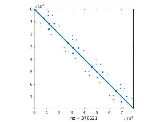
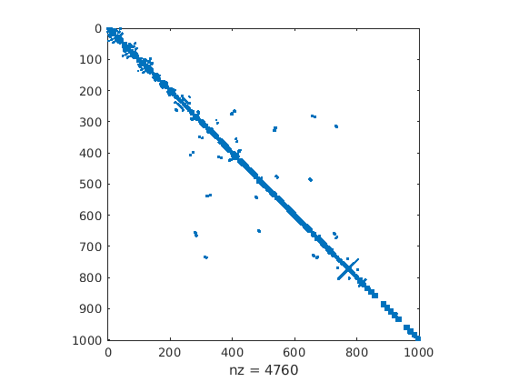
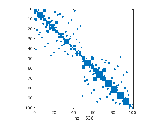
Define the system matrix .
|
|
Figure 2. Structure of
at various magnification factors
|
The data contains
points in ,
, and
line segments
defined by 2 endpoints. The total number of degrees of freedom is
.
Of the possible
linkages between points in the structure, only
are present.
∴ |
m=3*NX; [NX NX^2 NL m m^2] |
|
(5) |
The matrix can be formed by loops
over the trusses as shown in the algorithm below.
;
;
|
|
Define a function to carry out the assembly process in
dimensions that returns a full matrix .
∴ |
function assembleK(d,L,X)
  NL = size(L)[1]; n=maximum(L); m=d*n; K=zeros(m,m)
  for k=1:NL
    i=L[k,1]; j=L[k,2]
    l=X[j,1:d]-X[i,1:d]; l=l/norm(l)
    p=d*(i-1); q=d*(j-1); P=l*l'
    for id=1:d
      for jd=1:d
        K[p+id,p+jd] = K[p+id,p+jd] - P[id,jd]
        K[p+id,q+jd] = K[p+id,q+jd] + P[id,jd]
        K[q+id,p+jd] = K[q+id,p+jd] + P[id,jd]
        K[q+id,q+jd] = K[q+id,q+jd] - P[id,jd]
      end
    end
  end
  return K
end; |
The above has been precomputed for the Eiffel Tower model. It is
wasteful, and often impossible due to memory constraints, to store
the entire matrix of possible couplings between points
()
since most of the matrix would consist of zero entries. Rather, only
the nonzero elements corresponding to the linked nodes are stored
through what is known as a sparse matrix. There are various
techniques to store sparse matrices, one of which is the
coordinate format defined by a vector of row indices , a vector of column indices
and a vector of values such that the
element of the matrix
is
The following instructions load the sparse representation of .
∴ |
dfile = matopen(ddir*"/KCOO.mat"); |
∴ |
flrows=read(dfile,"rows"); |
∴ |
flcols=read(dfile,"cols"); |
∴ |
vals=read(dfile,"vals"); |
∴ |
rows=zeros(Int64,nz,1); cols=zeros(Int64,nz,1); |
∴ |
for l=1:nz
  rows[l] = floor(Int64,flrows[l])
  cols[l] = floor(Int64,flcols[l])
end |
∴ |
[minimum(rows) maximum(rows) minimum(cols) maximum(cols)] |
∴ |
K=sparse(rows[:,1],cols[:,1],vals[:,1]); |
∴ |
[rows[56] cols[56] vals[56]] |
|
(8) |
1.3Utility routines
Draw the deformed structure in figure
, given node
coordinates ,
displacements ,
,
skipping nodes
(to reduce drawing time).
∴ |
function drawXu(X,u,L,ks,nf)
  fig=figure(nf); ax = fig[:add_subplot](1,1,1,projection="3d")
  NX,d = size(X); NL,ns = size(L)
  U=reshape(u,d,NX)'
  for k=1:ks:NL
    i=L[k,1]; j=L[k,2]
    x=[X[i,1]+U[i,1] X[j,1]+U[j,1]]'
    y=[X[i,2]+U[i,2] X[j,2]+U[j,2]]'
    z=[X[i,3]+U[i,3] X[j,3]+U[j,3]]'
    ax[:plot](x,y,z,"k")
  end
  axis("equal")
end; |
Draw the deformed structure in figure
, given node
coordinates ,
displacements ,
,
skipping nodes.
∴ |
function drawXU(X,U,L,ks,nf)
  fig=figure(nf); ax = fig[:add_subplot](1,1,1,projection="3d")
  NX,d = size(X); NL,ns = size(L)
  for k=1:ks:NL
    i=L[k,1]; j=L[k,2]
    x=[X[i,1]+U[i,1] X[j,1]+U[j,1]]'
    y=[X[i,2]+U[i,2] X[j,2]+U[j,2]]'
    z=[X[i,3]+U[i,3] X[j,3]+U[j,3]]'
    ax[:plot](x,y,z,"k")
  end
  axis("equal")
end; |
Here are instructions to draw the structure with no node
displacement.
These are instructions to draw the structure with displacements
along the
direction proportional to the
coordinate
∴ |
U=zeros(NX,3); c=0.25; U[:,1]=c*X[:,3]; |
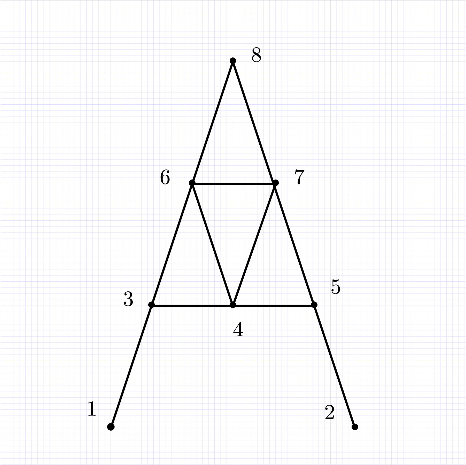
1.4Simplified “A” model
The full Eiffel Tower model is quite complex. It is convenient to build
familiarity with modeling binary interactions using the much simpler
two-dimensional ()
8-node model shown in Fig. 3
 |
|
Figure 3. “A” model of Eiffel
tower
|
1.5Enforcing boundary conditions
When structures are attached to their
environment, boundary conditions have to be enforced in the linear
system .
A common technique is set the diagonal element of
for the node subjected to boundary
conditions to a large value such that
it effectively decouples from the system, and set
where is the
desired boundary value.
∴ |
i=500; B=1.0e9; K[i,i]=B; f[i]=B*0.2; |
∴ |
i=501; B=1.0e9; K[i,i]=B; f[i]=B*0.2; |
∴ |
i=502; B=1.0e9; K[i,i]=B; f[i]=B*0.2; |
∴ |
i=1000; B=1.0e9; K[i,i]=B; f[i]=B*0.2; |
∴ |
i=1001; B=1.0e9; K[i,i]=B; f[i]=B*0.2; |
∴ |
i=1002; B=1.0e9; K[i,i]=B; f[i]=B*0.2; |
2Time-dependent case
Newton's second law of motion states that the rate of change of an
object's momentum is equal to the externally applied forces. For a
single point mass moving along the -axis,
this is stated as
where is the point mass position, its
velocity, its mass (inertia, resistance
to change of motion), and the external
force. If the mass remains constant (not the case for systems that
eject/intake matter such as stars or rockets, neither for motion at
speeds close to the speed of light when the resistance to change of
motion goes to infinity), the familiar
law results.
For binary interaction models (Eiffel tower model, “A”
model) a common technique to account for inertia is the so-called
“lumped mass” model in which the mass of a truss is
allocated as point masses concentrated at the nodes, i.e., the truss
end-points. Assembly of contributions from all trusses leads to the
system
The advantage of a lumped-mass model is that
is a diagonal matrix. Project this system onto the orthonormal basis
with the projection of the system
trajectory onto .
Obtain
with ,
,
.
While
are large and require sparse representations,
are small and can be stored as full matrices. The above second-order ODE
system with equations can be rewritten as
a first-order system with
equations
The notation is meant to signify the solution of
the system
to find by some numerical algorithm,
e.g.,
or
decomposition. Since the lumped mass matrix
does not vary in time, the decomposition is computed just once, prior to
time iteration, .
At some given time ,
is found by solving the triangular system
In the following problems assume a harmonically time-varying external
force
with a force
amplitude taken to be
in dimensions. This corresponds to a
force increasing with structure height ,
and is a reasonable model of structure interaction with a wind.
3Tasks
-
Construct
by distributing the mass of a truss to its endpoints. Assume trusses
have the same linear density ,
such that the mass of a truss is
-
Construct an algorithm to integrate the ODE system
by use of:
-
Track 1
-
The fourth-order Runge-Kutta algorithm from H09;
-
Track 2
-
The fourth-order predictor-corrector algorithm using
Adams-Bashforth as a predictor and Adams-Moulton as a
corrector (see H09).
-
Let be the
solution obtained above for
containing singular vectors of . Construct a convergence study through
plots of the error
in the
norms. In the above is taken as some
large number of modes, and .
The choice of is dictated by
computational constraints, i.e., the largest amount of execution
time on a specific machine. For a typical laptop .