MATH661 Project 3 - Operator approximation in Sturm-Liouville eigenbasis

MATH661 Project 3 - Operator approximation in Sturm-Liouville eigenbasis

Posted: 11/30/22

Due: 12/03/22 11:55PM (First Draft), 12/07/22, 5:00PM (Final Draft)

$\circ$ Julia SpecialFunctions package installation (only needs to be invoked once, will be used in this assignment)

This serves both as your final project and final examination. The topic you are exploring is the use of problem-specific bases. In the project, an academic analytical cyclindrical function basis is used to exemplify the idea, but in practice bases are extracted from the problem itself. The monograph by Patera and Rozza in the MATH661/bibliography directory presents a full treatment. This final examination is meant to be completed in 3-9 hours. Read through the Introduction prior to December 3, add the SpecialFunctions package to your Julia environment, and complete a first draft during the regularly scheduled Final Examination time of on Saturday, Dec. 3. Comments on the first draft will be returned by 3:00PM on Monday Dec. 5. Address the comments and submit a second, final draft during the reading day, Dec. 7.

1Introduction

1.1Sturm-Liouville eigenfunctions

It is traditional to introduce the main concepts in operator approximation using the monomial basis $ℳ = {1, t, t^{2}, \dots}$ in which integration and differentiation operations are simple to carry out. However, in numerical work algorithm conditioning, stability, and accuracy are more important than easy-to-use analytical formulas. This final project brings together all main course concepts to construct approximation procedures for problems that are naturally stated in the eigenfunctions of a Sturm-Liouville problem for an orthogonal, curvilinear coordinate system.

1.1.1Regular Sturm-Liouville problems

The regular Sturm-Liouville problem (SLP) is to find $y : [a, b] \to ℝ$ , twice differentiable that satisfies

L (y) = \frac{d}{d x} [w (x) y^{'}] + [q (x) + λ p (x)] y = 0,

(1)

with the two-point boundary value conditions $V (y) = 0$

A_{1} y (a) + B_{1} y^{'} (a) = 0,

A_{2} y (b) + B_{2} y^{'} (b) = 0 .

The functions $p, q$ are continuous and $w$ is differentiable. The SLP is linear in operator $L$ and boundary conditions $V .$ When $w (x) > 0$ and $p (x) > 0$ the SLP is said to be regular. A singular SLP results when $w (x) = 0$ for some $x \in [a, b]$ .

1.1.2Physical conservation laws

The ubiquity of SLPs is due to physics being naturally expressed through a small set of conservation laws, e.g., mass, momentum, energy, and electrical charge in classical physics (additional quantum conservation laws arise from quantum mechanics). Consider the familiar statement from mechanics

𝑭 = m 𝒂,

more properly written as

\frac{d}{d t} (𝑯) = 𝑭,

stating that the rate of change of a point mass's momentum $𝑯$ is due to the sum of applied forces $𝑭$ . In the absence of any external forces the momentum is conserved

\frac{d}{d t} (𝑯) = 0 \Rightarrow 𝑯 = constant .

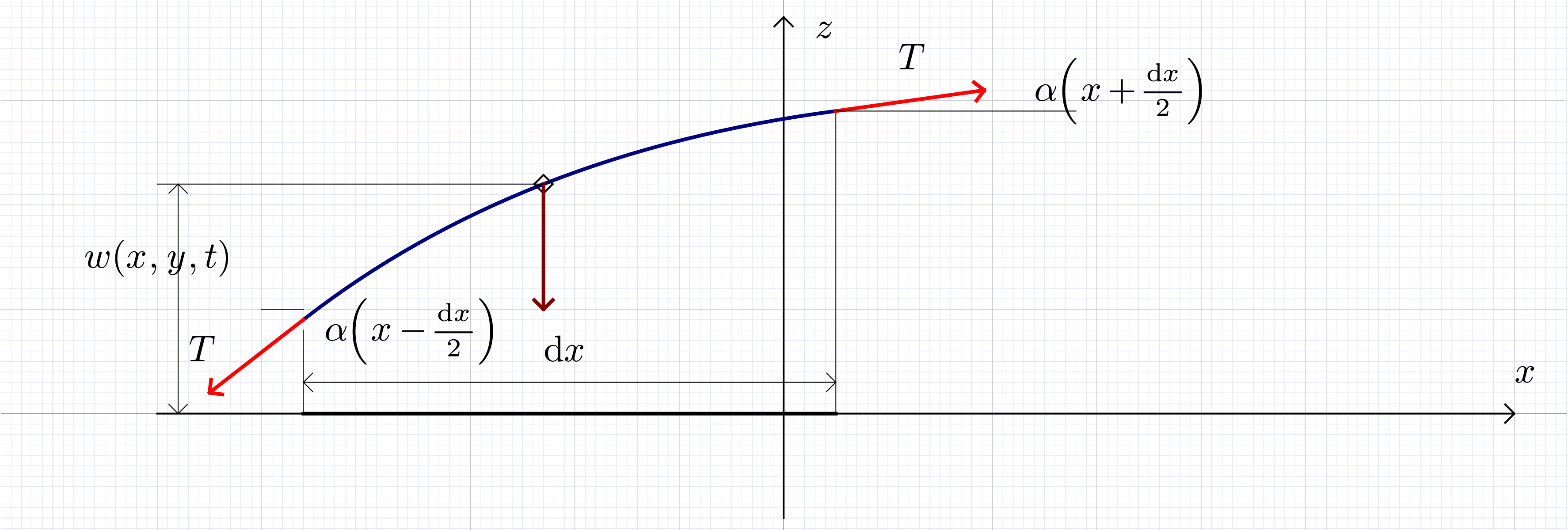
When applied to continua, conservation laws lead to PDEs, for example the motion of a drumhead membrane. An infinitesimal portion of membrane of area $d A = d x d y$ has mass $d m = ρ d A$ and is brought out of its equilibrium position by small displacement $w (x, y, t)$ along the $z$ -axis, such that the tangent makes angle $α ≅ \sin α ≅ \tan α = \partial w / \partial x$ . The membrane is stretched from its equilibrium position by tension $T$ , and the resultant force on the infinitesimal portion is

T [\frac{\partial w}{\partial x} (x + \frac{d x}{2}) - \frac{\partial w}{\partial x} (x - \frac{d x}{2})] ≅ T \frac{\partial^{2} w}{\partial x^{2}} .

A similar argument along the $y$ -axis then gives the wave equation

w_{t t} = c^{2} div (grad w) = c^{2} \nabla \cdot (\nabla w) = c^{2} (w_{x x} + w_{y y}),

with $w_{x x} = \partial^{2} w / \partial x^{2}$ , etc., and $c^{2} = T / ρ$ .

For a square-shaped drumhead with edge-length $a$ that is pinned along its perimeter, separation of variables $w (x, y, t) = X (x) Y (y) T (t)$ then leads to

\frac{1}{c^{2}} \frac{T^{''}}{T} = \frac{X^{''}}{X} + \frac{Y^{''}}{Y} = - \frac{ω^{2}}{c^{2}}

and three SLPs, e.g., along $x$

X^{''} + n^{2} X = 0, X (0) = X (a) = 0 .

The eigenfunctions in this case are the familiar trig-functions $\sin (n π x / a)$ . These eigenfunctions play a fundamental role in problems stated in Cartesian coordinates, as exemplified by Fourier transforms.

1.1.3Differential operators in curvilinear coordinates

Consider now a circular-shaped of radius $r = a$ drum pinned along its perimeter, in which case it is convenient to carry out separation of variables in polar coordinates $w (r, θ, t) = R (r) Θ (θ) T (t)$ . The wave equation in polar coordinates

w_{t t} = c^{2} \nabla \cdot (\nabla w) = c^{2} [w_{r r} + \frac{1}{r} w_{r} + \frac{1}{r^{2}} w_{θ θ}],

then leads to

\frac{1}{c^{2}} \frac{T^{''}}{T} = \frac{R^{''}}{R} + \frac{1}{r} \frac{R^{'}}{R} + \frac{1}{r^{2}} \frac{Θ^{''}}{Θ} = - \frac{ω^{2}}{c^{2}},

and assuming rotational symmetry around the $z$ -axis, $Θ^{''} = 0$ , gives two ODEs

T^{''} + ω^{2} T = 0 \Rightarrow T (t) = A \cos (ω t) + B \sin (ω t),

for which initial conditions are given, and the SLP

R^{''} + \frac{1}{r} R^{'} + k^{2} R = 0, R (0) finite, R (a) = 0, k^{2} = \frac{ω^{2}}{c^{2}} .

(2)

The ODE has general solution

R (r) = A J_{0} (k r) + B Y_{0} (k r),

and imposing boundary conditions leads to $B = 0$ (to maintain finite $R (0)$ ) and

J_{0} (k a) = 0,

(3)

with a denumerable set of solutions $k_{n}$ , $n = 1, 2, \dots$ , the eigenvalues of the SLP, $k_{1} < k_{2} < \dots$ . The corressponding eigenfunctions are $y_{n} (r) = J_{0} (k_{n} r_{})$ , and can be evaluated in Julia through the besselj0() function. SLP eigenfunctions are orthogonal with respect to the scalar product

(f, g) = \int_{0}^{a} p (r) f (r) g (r) d r,

i.e.

m \neq n \Rightarrow \int_{0}^{a} p (r) J_{0} (k_{m} r) J_{0} (k_{n} r) d r = 0 .

The Bessel function has an asymptotic approximation

J_{0} (x) ≅ \sqrt{\frac{2}{π x}} \cos (x - \frac{π}{4}),

useful in initial approximation of the eigenvalues from (3). Another useful result is

\frac{d}{d x} J_{0} (x) = - J_{1} (x),

evaluated by the besselj1() Julia function.

In the following length units are chosen such that the drumhead has radius $a = 1$ .

2Track 1 & 2 common problems

Use Newton's method to find the first $n = 64$ eigenvalues by solving (3) numerically to six-digit accuracy (relative error $ε < 10^{- 6}$ ). Plot the eigenvalues. Plot the $j = 1, 2, 4, 8, 16, 32$ eigenfunctions $y_{j} (r)$ . Comment on the basis functions by comparison, say, to the monomial basis ${1, r, r^{2}, \dots}$ .
Identify in (2) the functions $w, r, p$ from the general formulation of a SLP (1). Verify eigenfunction orthogonality numerically through the approximation

$(y_{m}, y_{n}) = \int_{0}^{1} p (r) y_{m} (r) y_{n} (r) d r ≅ 𝒚_{m}^{T} 𝑷 𝒚_{n}$ (4)

where $𝒚_{m}$ is a sampling of the eigenfunction at nodes $𝒓 = [r_{i}] \in ℝ^{N}$
$h = 1 / N, r_{i} = i h, i = 1, \dots, N,$
and the scalar product weight $p (r)$ determines the diagonal matrix $𝑷 = diag (p (𝒓))$ . The approximation (4) is a (right) Darboux sum, or approximation of the integral by a piecewise constant function. Plot the orthogonality error $|| 𝒀^{T} 𝑷 𝒀 ||$ with increasing $N = 2^{q}$ , $q = 3, \dots, 12$ in log coordinates.

3Track 1 problems

3. Increase the accuracy of scalar product evaluation by replacing (4) by:

composite midpoint integration;
composite trapezoid integration;
composite Simpson integration.

For each of the above, plot the orthogonality error.

4. Determine the expansion of the initial condition $w (0, r) = 1 - r$ on the Bessel function bases containing $P = 2^{r}$ , $r = 4, 5, 6, 7$ vectors.

4Track 2 problems

3. Increase the accuracy of scalar product evaluation by replacing (4) by composite Gauss-Legendre quadrature of with 2 and 3 points per subinterval. For each of the above, plot the orthogonality error.

4. Generate Gauss quadrature formulas over the entire interval of orders $q = 4, 6, 7, 8$ by orthogonalization of the monomial basis ${1, r, r^{2}, \dots}$ with respect to the scalar product (3), finding the roots of the polynomials of degree $q$ , and determining the appropriate quadrature coefficients

\int_{0}^{1} p (r) f (r) d r = \sum_{i = 1}^{q} c_{i} f (r_{i}) .