This homework serves as an introduction to number approximation techniques and a familiarization with homework drafting and submission procedures. No grade points are awarded, but comments on proper assignment drafting are returned.

1. Construct a convergence plot in logarithmic coordinates of the Stern continued fraction

   ${\displaystyle \frac{\pi }{2}=1-}$

   Identify the terms in the general expression of a continued fraction

   ${\displaystyle F_n=b_0+\stackrel{n}{\underset{k=1}{\text{K}}}\frac{a_k}{b_k}.}$

   Compare with the additive approximation of the Leibniz series

   ${\displaystyle \frac{\pi }{4}=1-\frac{1}{3}+\frac{1}{5}-\frac{1}{7}+\frac{1}{9}-\dots .,}$

   Estimate the rate and order of convergence for both approximations.

   Solution. (a) Identification of terms: the first few terms are

   ${\displaystyle b_0=1,b_1=3,b_2=1,b_3=3,b_4=1,b_5=3,}$ ${\displaystyle a_1=-1\cdot 1,a_2=-2\cdot 3=-6,a_3=-1\cdot 2=-2,a_4=-4\cdot 5=-20,a_5=-3\cdot 4=-12.\left(b\right)}$

   With $l=kmod2$, $t=2l-k$, $k\in \mathbb{N}$, obtain $b_k=1+2l$, and $a_k=t(1-t)$ for $k>1$. (c)

   $\circ$

   Figure 1. Comparison of convergence of Leibniz series ($\times$) and Stern continued fraction ($•$). (d)

   (e,f) Calculate log of absolute error $e_k=|L_k-\pi /4|$ of Leibniz partial sums.

   ∴	N=200; n=20:20:N;

   ∴	function Leibniz(n) k=0:n sum((-1).^k ./ (2*k.+1)) end;

   ∴	errL=log.(abs.(Leibniz.(n) .- π/4));

   ∴

   (g) Define functions that return terms $a_k,b_k$ in the Stern continued fraction. (h,i)

   ∴	function aS(k) if k<2 return -1 end l = k % 2; t=2*l-k return t*(1-t) end;

   ∴	function bS(k) l = k % 2 return 1+2*l end;

   ∴	[aS.(1:5) bS.(1:5)]

   ${\displaystyle \left[\begin{array}{cc}-1& 3\\ -6& 1\\ -2& 3\\ -20& 1\\ -12& 3\end{array}\right]}$

   (1)

   ∴

   (j) Define a function to evaluate a continued fraction. The arguments are themselves functions to compute the continued fraction coefficients.

   ∴	function ContFrac(n,a,b) F = 0 for k=n:-1:1 F = a(k)/(b(k)+F) end return b(0)+F end;

   ∴	ContFrac.(50:50:250,aS,bS)

   ${\displaystyle \left[\begin{array}{c}1.55547258345075\\ 1.5630394501077056\\ 1.565603654293689\\ 1.5668937453140812\\ 1.5676703732493937\end{array}\right]}$

   (2)

   Calculate log of absolute error of truncated Stern continued fractions.

   ∴	errS=log.(abs.(ContFrac.(n,aS,bS) .- π/2));

   Construct plot and save a high-quality rendition as an encapsulated postscript file. Insert image into the figure environment.

   ∴	clf(); plot(log.(n),errL,"-o",log.(n),errS,"-x"); xlabel("log(n)"); ylabel("log(err)"); title("Convergence commparison"); grid("on"); plot([3,4],[-5,-7],"-"); plot([3,4],[-5,-6],"-");

   ∴	savefig(homedir()*"/courses/MATH661/homework/H00/Fig01.eps")

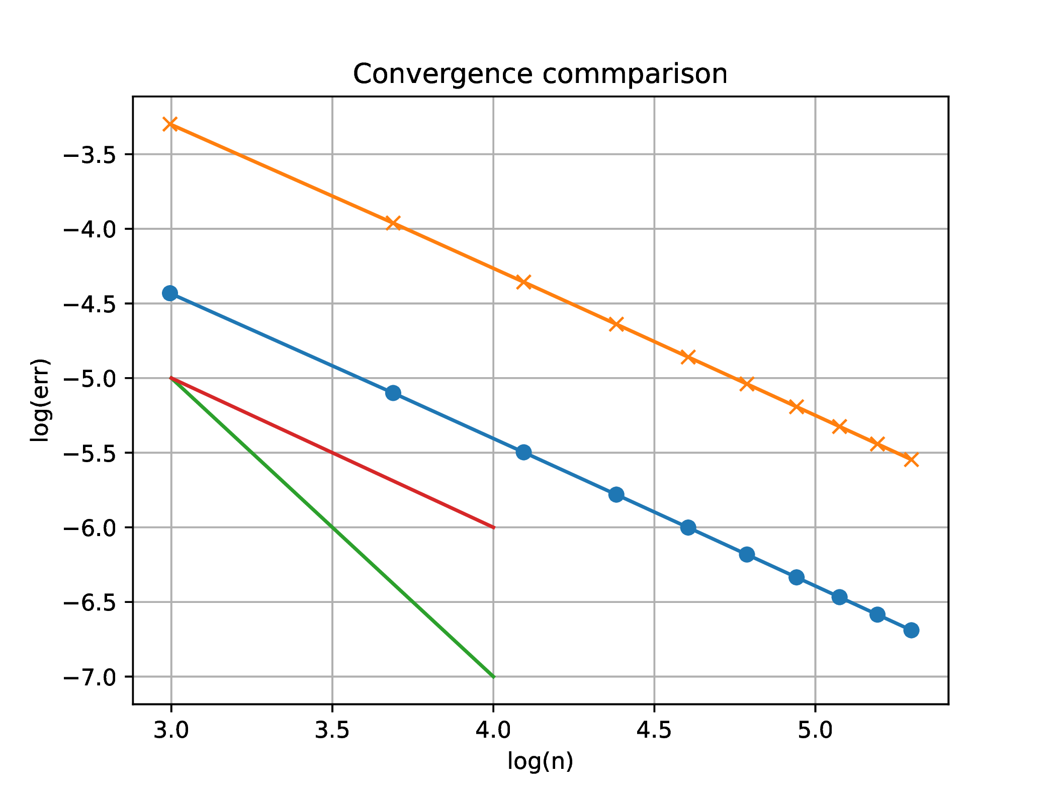
   $\circ$For large enough $n$, the distance of a term sequence to the limit $d_n=|x_n-x|$ satisfies

   ${\displaystyle d_{n+1}\cong s{d}_n^q,d_n\cong s{d}_{n-1}^q,}$

   whence

   ${\displaystyle \frac{d_{n+1}}{d_n}\cong {\left(\frac{d_n}{d_{n-1}}\right)}^q\Rightarrow q\cong \frac{\log d_{n+1}-\log d_n}{\log d_n-\log d_{n-1}},}$

   and then

   ${\displaystyle s\cong d_{n+1}/d_n^q.}$

   Results are presented in the following table, with both sequences exhibiting close to linear convergence. (k)

   Leibniz Stern Rate $s$ 0.963 0.938 Order $q$ 0.995 0.990

   Table 1. Convergence behavior of Leibniz series and Stern continued fraction (d)

   Compute data needed for rate and order of convergence estimation. The Stern sequence exhibits two subsequences (suggested by the modulo 2 dependence of the coefficients), and one of these is chosen for convergence estimation, i.e., the even-indexed one.

   ∴	dL=abs.(Leibniz.(N:N+2) .- π/4); dS=abs.(ContFrac.(N:2:N+4,aS,bS) .- π/2);

   ∴

   Define a function to estimate rate and order of convergence from error data

   ∴	function SeqConv(d) q = (log(d[3])-log(d[2]))/(log(d[2])-log(d[1])) s = d[3]/d[2]^q return [s; q] end;

   ∴	[SeqConv(dL) SeqConv(dS)]

   ${\displaystyle \left[\begin{array}{cc}0.9627156921670497& 0.9378213813852142\\ 0.9950618292587109& 0.990208098475882\end{array}\right]}$

   (3)

   ∴

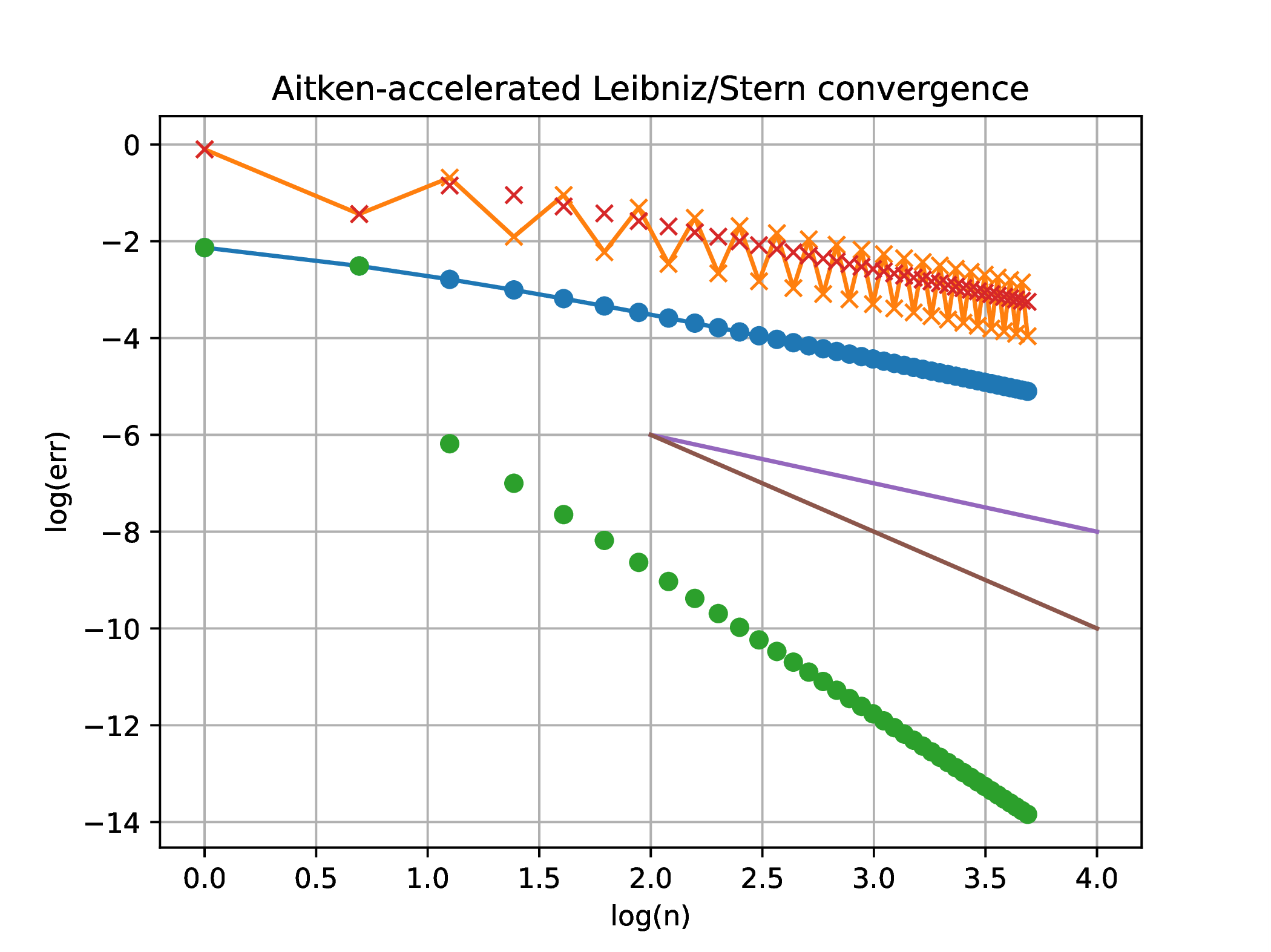
2. Apply convergence acceleration to both the above approximations involving $\pi$. Construct the convergence plot of the accelerated sequences, and estimate the new rate and order of convergence.

   Solution. (a) Since both the Leibniz and the Stern sequences exhibit close to linear convergence, Aitken acceleration is applicable (though not guaranteed to provide faster convergence since it is an extrapolation).

   $•$

   Figure 2. Aitken acceleration of Leibniz and Stern sequences. While second-order convergence is obtained for the Leibniz sequence, the modulo 2 alternating coefficients yield no increase in order of convergence for the Stern sequence (k).

   Generate terms in the Leibniz, Stern sequences

   ∴	N=40; n=1:N; L=Leibniz.(n); S=ContFrac.(n,aS,bS);

   ∴

   Define a function that carries out Aitken acceleration. (j)

   ∴	function Aitken(x) n=maximum(size(x)); a=copy(x); for k=3:n Δx = x[k] - x[k-1] Δ2x = x[k] - 2*x[k-1] + x[k-2] a[k] = x[k] - Δx^2/Δ2x end return a end;

   ∴	AL = Aitken(L); AS = Aitken(S);

   ∴

   Construct plot of errors for both original and accelerated sequences

   ∴	errL=log.(abs.(L .- π/4)); errAL=log.(abs.(AL .- π/4));

   ∴	errS=log.(abs.(S .- π/2)); errAS=log.(abs.(AS .- π/2));

   ∴	clf(); plot(log.(n),errL,"-o"); plot(log.(n),errS,"-x"); plot(log.(n),errAL,"o"); plot(log.(n),errAS,"x"); xlabel("log(n)"); ylabel("log(err)"); title("Aitken-accelerated Leibniz/Stern convergence"); grid("on"); plot([2,4],[-6,-8],"-"); plot([2,4],[-6,-10],"-");

   ∴	savefig(homedir()*"/courses/MATH661/homework/H00/Fig02.eps")

   ∴

3. Completely state the mathematical problem of taking the $n^{\mathrm{th}}$ root of a positive real, $n\in \mathbb{N}$. Find the absolute and relative condition numbers.

   Solution. Within the framework of defining a mathematical problem as a function $f:X\to Y$ (l), the choices

   ${\displaystyle f\left(x\right)=x^{1/n},}$

   with $X={ℝ}_{+}=(0,\infty )$, $Y=ℝ$, can be made. Other options (m) include $X={ℝ}_{+}\times \mathbb{N}$ treating $n$ as a variable or considering the framework of multivalued functions (regularized by cuts in the complex plane) for which $Y=ℂ$. Since $f$ is differentiable, the absolute condition number is given by the derivative

   ${\displaystyle {\hat{\kappa }}_f\left(x\right)=\frac{1}{n}{x}^{1/n-1}.}$

   The relative condition number is then

   ${\displaystyle {\kappa }_f\left(x\right)=\frac{1}{n}\frac{x^{1/n-1}}{x^{1/n}}x=\frac{1}{n}.}$

4. Completely state the mathematical problem of finding the roots of the cubic polynomial $p\left(x\right)=x^3+px+q$, using the Cardano [2] formula. Find the absolute and relative condition numbers.

   Solution. Assuming $(p,q)\in {ℝ}^2$, then one real root is obtained as

   ${\displaystyle f(p,q)=\sqrt[3]{g(p,q)}+\sqrt[3]{h(p,q)},}$

   where

   ${\displaystyle g(p,q)=-\frac{q}{2}+\sqrt{D(p,q)},h(p,q)=-\frac{q}{2}-\sqrt{D(p,q)},D(p,q)=\frac{q^2}{4}+\frac{p^3}{27},\left(n\right)}$

   and $D(p,q)$ is assumed to be positive. In this case $X={ℝ}^2$, $Y=ℝ$, though in general (m) $p,q$ might be complex. The function $f$ is a composition of differentiable functions, so the condition number may be evaluated as the norm of the gradient

   ${\displaystyle {\hat{\kappa }}_f=||\nabla f||=\frac{1}{3}||g^{-2/3}\nabla g+h^{-2/3}\nabla h||.}$

   Further calculation gives

   ${\displaystyle \nabla g=\left[\begin{array}{l}0\\ -1/2\end{array}\right]+\frac{1}{2}{D}^{-1/2}\nabla D,\nabla g=\left[\begin{array}{l}0\\ -1/2\end{array}\right]-\frac{1}{2}{D}^{-1/2}\nabla D,}$ ${\displaystyle \nabla D=\left[\begin{array}{l}{p}^2/9\\ q/2\end{array}\right].}$

   The relative condition number can be stated

   ${\displaystyle {\hat{\kappa }}_f=\frac{||\nabla f||}{\left|f\right|}{(p^2+q^2)}^{1/2},\left(n\right)}$

   choosing the 2-norm in $X$.

5. Completely state the mathematical problem of solving the initial value problem for an ordinary differential equation of first order. Use Lyapunov exponents [1] to find the absolute condition number.

   Solution. For the initial value problem (IVP) expressed in autonomous form (always possible) (l)

   ${\displaystyle y^{\text{'}}=s\left(y\right),y\left(0\right)=y_0,}$

   the problem inputs are the slope function $s$ that has to be Lipschitz continuous, $s\in C^{k,1}$ to obtain a unique solution (l) and the initial value $y_0\in ℝ$. The definition of the mathematical problem is then $X=C^{k,1}\times ℝ$, $Y=C$. In this formulation the condition number requires the definition of the derivative of a function (i.e., the solution $y$) with respect to another function (the slope $s$). (o)

   Since the Lyapunov exponent $L$ quantifies the rate of separation of trajectories upon infinitesimal perturbation of the initial condition $\delta y_0$, in the simpler case of considering $s$ fixed, the condition number is identical to the Lyapunov exponent, $\hat{\kappa }=e^L$.

Bibliography