Solution. Proofs of the
Hölder inequality can use approaches from elementary algebra,
analysis, or measure theory. However, the interest here is
interpreting the Hölder inequality in the context of linear
algebra. Study the following solution carefully to see how an
operator was identified, represented by a matrix, and then the
tools introduced to measure the magnitude of vectors and matrices
(i.e., norms) were used to establish the Hölder inequality.
Compare with your submitted solution, and establish links between
the fields of mathematics used in your proof to the linear algebra
proof presented here.
Introduce vectors ,
and matrices
defined as
Notice that ,
is a vector with components .
The Hölder inequality can now be stated in matrix-vector form
as
The inequality is true for either ,
or .
For the remaining case of ,
,
rescale vectors such that ,
and restate Hölder inequality,
Use the matrix norm property .
The one-norm of a matrix is the largest of the one-norms of its
columns (e.g., Trefethen & Bau, p.21), and since the columns
of contain a single non-zero
entry
since, otherwise, if then ,
contradiction. This leads to
Recall the graphical representation of unit-circles in various
vector norms, .
This is readily constructed by drawing an arc in the first
quadrant, that is subsequently rotated by
.
∴ |
function arc(p,m)
  u1 = LinRange(0,1,m);
  u2 = (1 .- u1.^p).^(1.0/p)
  return [u1 u2]'
end; |
∴ |
function R(θ)
  [cos(θ) -sin(θ); sin(θ) cos(θ)]
end; |
∴ |
clf(); m=90; c=["k" "b" "g" "r"]; axis("equal"); title("Unit circle in various p-norms"); |
∴ |
for p=1:4
  X=[R(0); R(π/2); R(π); R(3*π/2)]*arc(p,m);
  for i=1:2:7
    plot(X[i,:],X[i+1,:],c[p])
  end
end |
∴ |
prefix = homedir()*"/courses/MATH661/images/"; |
∴ |
savefig(prefix*"H02T2P1.eps"); |
 |
|
Figure 3. Visual data suggesting that
for ,
|