This homework introduces the fundamentals of additive approximation techniques in vector spaces. Read and understand the concepts in L04: Linear combinations in ${ℛ}_m$ and ${𝒞}^0[0,2\pi )$, in particular to the example presented in the text and in the code attached to L04: Figure 2. Additional Julia coding constructs are also introduced. Remember to always execute the code snippets within the lecture notes to understand Julia programming techniques.

1. Approximate $b\left(t\right)=t(\pi -t)(2\pi -t)$ on the interval $[0,2\pi )$ by the following series and study the convergence behavior of the solution. The pseudo-matrix $A\left(t\right)$ arising in the approximation is shown in each case

   1. Cosine series

      ${\displaystyle b\left(t\right)\cong \sum _{k=0}^n{x}_k\cos (kt),}$ ${\displaystyle A\left(t\right)=\left[\begin{array}{lllll}1& \cos \left(t\right)& \cos \left(2t\right)& \dots & \cos (nt)\end{array}\right],A:ℝ\to {ℝ}^{n+1}.}$

   2. Trigonometric series

      ${\displaystyle b\left(t\right)\cong \sum _{k=0}^n[x_k\cos (kt)+y_k\sin (kt)],}$ ${\displaystyle A\left(t\right)=\left[\begin{array}{llllllll}1& \cos \left(t\right)& \sin \left(t\right)& \cos \left(2t\right)& \sin \left(2t\right)& \dots & \cos (nt)& \sin (nt)\end{array}\right],A\left(t\right):ℝ\to {ℝ}^{2n+1}.}$

   3. Sine series

      ${\displaystyle b\left(t\right)\cong \sum _{k=1}^n{y}_k\sin (kt),}$ ${\displaystyle A\left(t\right)=\left[\begin{array}{llll}\sin \left(t\right)& \sin \left(2t\right)& \dots & \sin (nt)\end{array}\right],A:ℝ\to {ℝ}^n.}$

   4. Triangle wave series

      ${\displaystyle b\left(t\right)\cong \sum _{k=1}^n{z}_k{W}_k(t),}$ ${\displaystyle A\left(t\right)=\left[\begin{array}{llll}{W}_1\left(t\right)& W_2\left(t\right)& \dots & W_n(t)\end{array}\right],A:ℝ\to {ℝ}^n,}$

      with

      ${\displaystyle W_k\left(t\right)=1-4|\frac{1}{2}-⟦\frac{1}{4}+\frac{kt}{2\pi }⟧|,}$

      where $⟦x⟧$ is the fractional part of $x$, e.g., $⟦1.15⟧=0.15$.

   Solution. Sample $b\left(t\right)$ at points $t_j=(j-1)h_{}$, $j=1,2,\dots ,m$, with spacing $h=2\pi /m$, and let $𝒕$ denote the vector with components $t_j$. Let $p$ denote the number of columns in the $A\left(t\right)$ pseudo-matrix, i.e., the number of functions $u_k\left(t\right)$ entering into the approximation of $b\left(t\right)$ by the linear combination

   ${\displaystyle f_p\left(t\right)=\sum _{k=1}^p{c}_k{u}_k\left(t\right).}$

   (1)

   Table 1 defines $c_k$, $u_k\left(t\right)$ for each of the four cases, with $k=1,2,\dots ,p$. Case $b$ also conforms to this pattern since the presence of both $\cos (kt)$ and $\sin (kt)$ suggests the use of complex numbers

   ${\displaystyle b_n\left(t\right)=\sum _{k=0}^n[x_k\cos (kt)+y_k\sin (kt)]=\frac{1}{2}\sum _{k=0}^n[x_k(e^{ikt}+e^{-ikt})-i{y}_k(e^{ikt}-e^{-ikt})]\Rightarrow }$

   ${\displaystyle b_n\left(t\right)=\frac{1}{2}[\sum _{k=0}^n(x_k-i{y}_k)e^{ikt}+\sum _{k=0}^n(x_k+i{y}_k)e^{-ikt}]=\frac{1}{2}[p_n\left(t\right)+q_n\left(t\right)].}$

   As expected for $b_n\left(t\right)\in ℝ$, $p_n\left(t\right),q_n\left(t\right)\in ℂ$ are complex conjugates

   ${\displaystyle {\bar{p}}_n\left(t\right)=\sum _{k=0}^n\overline{(x_k-i{y}_k)}\overline{e^{ikt}}=\sum _{k=0}^n(x_k+i{y}_k)e^{-ikt}=q_n\left(t\right),}$

   hence only one need be computed and the expression

   ${\displaystyle f_p\left(t\right)=2\mathrm{Re}\{\sum _{k=1}^p{c}_k{e}^{-i(k-1)t}\}}$

   is obtained, indeed conforming to the same pattern as the other cases.

   Case $c_k$ $u_k\left(t\right)$ $a$ $y_k$ $\cos ((k-1)t)$ $b$ $x_k+i{y}_k$ $e^{-i(k-1)t}$ $c$ $y_k$ $\sin (kt)$ $d$ $z_k$ $W_k\left(t\right)$

   Table 1. Coefficient, basis function definitions.

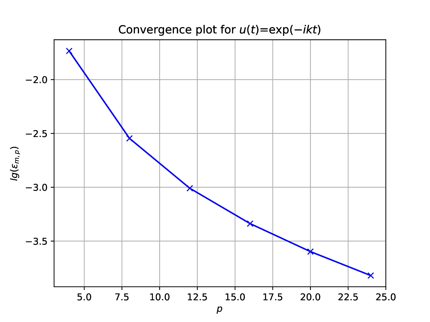
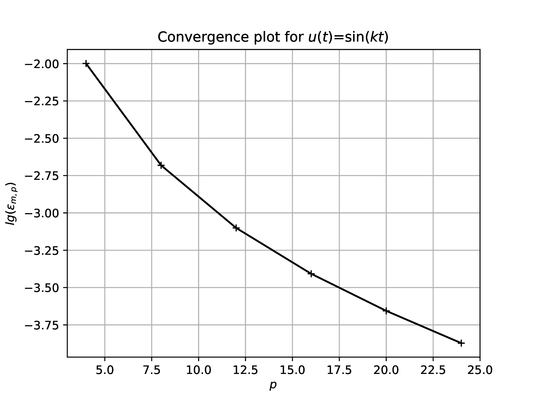
   Problem solution consists of the following steps, leading to results in Fig. 1.

   $\circ$Define $b\left(t\right)$ and the basis functions $u_{\alpha }(k,t)$, $\alpha \in \{a,b,c,d\}$ to be investigated.

   ∴	b(t)=t*(pi-t)*(2*pi-t);

   ∴	ua(k,t)=cos((k-1)*t);

   ∴	i=1im; ub(k,t)=exp(-i*(k-1)*t);

   ∴	uc(k,t)=sin(k*t);

   ∴	ud(k,t)=1-4*abs(0.5-floor(0.25+k*t/2/pi));

   ∴

   $\circ$Define a function to compute the error in approximating $b\left(t\right)$ by a series with $p$ terms with coefficients determined by sampling at $m$ points

   ${\displaystyle E(m,p)=||f_p\left(𝒕\right)-b\left(𝒕\right)||/||b\left(𝒕\right)||,}$

   with $b\left(𝒕\right),f_p\left(𝒕\right)\in {ℝ}^m$ vectors obtained by sampling $b\left(t\right),f_p\left(t\right)$ at $𝒕\in {ℝ}^m$. With $𝒄\in {ℝ}^p$ the vector with components $c_k$, $f_p\left(𝒕\right)$ is evaluated by the matrix-vector product

   ${\displaystyle f_p\left(𝒕\right)=A\left(𝒕\right)𝒄.}$

   Julia (as most modern languages) allows passing a function name as an argument allowing efficient numerical experiments with the different approximation bases. Use this feature to write functions to:

   1. Set up the problem;

      ∴	function SetUp(m,p,u,b) h=2*pi/m; j=1:m; t=(j.-1)*h; A=u.(1,t) for k=2:p A = [A u.(k,t)] end bt = b.(t) return A,bt end;

      ∴

   2. Compute the error;

      ∴	function E(m,p,u,b,sc) A,bt = SetUp(m,p,u,b); c = A\bt; fp = sc*real(A*c) return norm(fp-bt)/norm(bt) end;

      ∴

   This implementation allows both error computation and investigation of the problem, e.g., number of independent columns in $𝑨$.

   ∴	E(72,16,ua,b)

   $1.0$

   ∴	A,bt = SetUp(72,16,ua,b); rank(A)

   $16$

   Note the close correspondence between the mathematical formulation and the coding, exemplified by the mathematical notation $b\left(𝒕\right)$ readily transcribed into Julia as bt=b.(t). Successful scientific computation relies on well-formulated mathematics that is then readily transcribed into pseudo-code or directly into a programming language. It is good coding practice to write short functions that carry out some specific task within an overall problem formulation, in this case problem formulation and computing the approximation error.

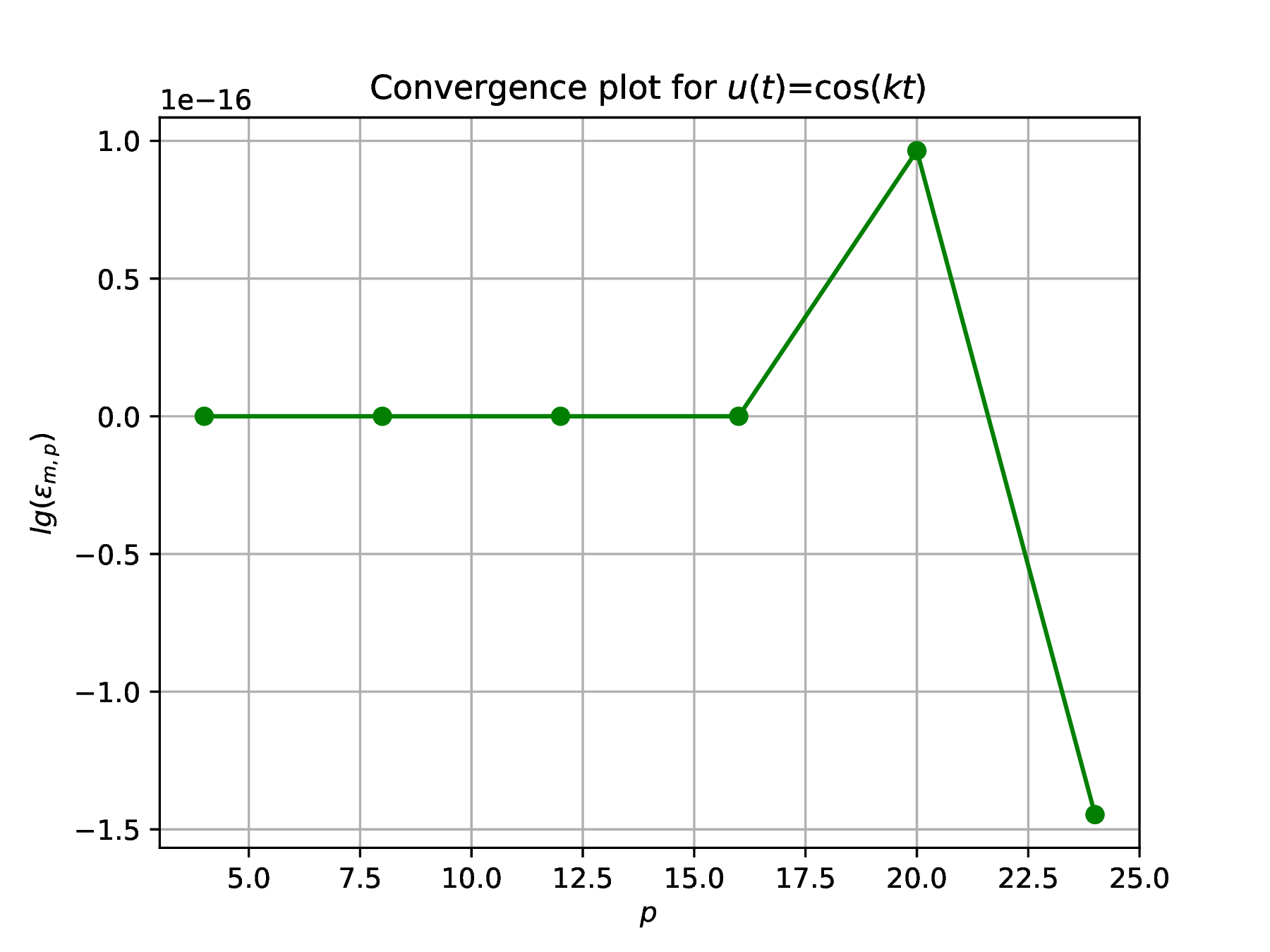
   $\circ$Test the error function by computing the coefficients for $v\left(t\right)=\cos \left(t\right)$ and $w\left(t\right)=\cos \left(t\right)+\cos \left(5t\right)$ using basis set $u_a(k,t)=\cos (kt)$. We should obtain zero error once enough terms are included.

   ∴	v(t)=cos(t); w(t)=cos(5*t);

   ∴	[E(10,1,ua,v,1) E(10,2,ua,v,1) E(10,3,ua,w,1) E(10,6,ua,w,1)]

   ${\displaystyle \left[\begin{array}{cccc}1.0& 7.975080594166061e-16& 1.0& 2.531698018113677e-16\end{array}\right]}$

   (2)

   ∴

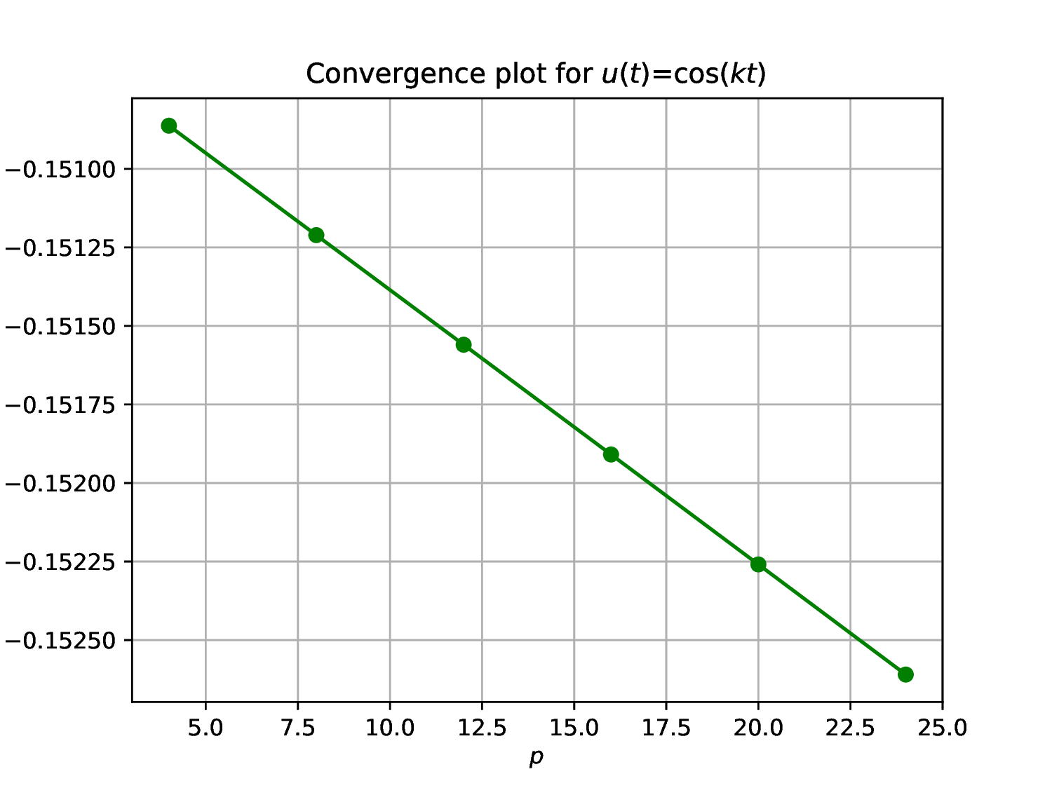
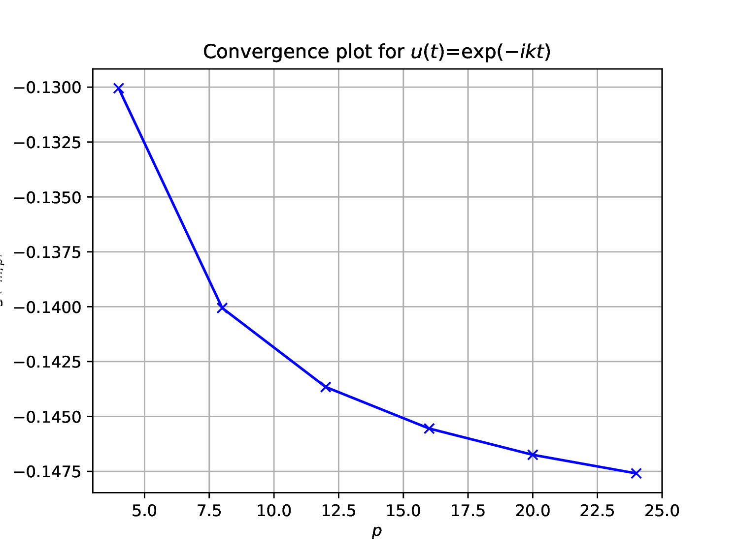
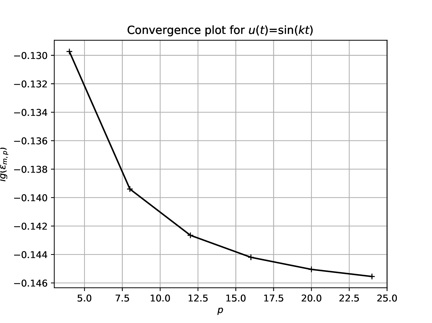
   $\circ$Define a function to construct a convergence plot by evaluating $E(m,p)$ on a of range $p$ values $\epsilon$

   ∴

   function plotE(m,prange,u,b,sc,ls,uname,fname) lgerr = zeros(length(prange)); i=1; minerr=eps(Float64) for p in prange err=max(E(m,p,u,b,sc),minerr); lgerr[i] = log10(err); i=i+1 end clf(); plot(prange,lgerr,"-"*ls); xlabel(L"p"); ylabel(L"lg(\epsilon_{m,p})"); grid("on"); title(L"Convergence plot for $u(t)$="*uname) savefig(homedir()*"/courses/MATH661/homework/H02/"*fname*".eps") end;

   ∴

   Note: Besides the numerical arguments, a number of plot options are defined as arguments. This eliminates the drudgery of interactively setting file names, plot colors, etc. Two useful Julia coding techniques are: (1) string concatenation, "a"*"bc"="abc", (2) LaTeX inclusion, L"text $u(t)$= ".

   $\circ$Choose sufficient sample points to resolve the function $b\left(t\right)$, say $m=100$, and construct convergence plots for the four cases

   Note: “to resolve a function” means to sample at enough points to observe the fastest variations in the function graph.

   ∴	m=100; pr=4:4:24;

   ∴	plotE(m,pr,ua,b,1,"og",L"\cos(k t)","Fig1a");

   ∴	plotE(m,pr,ub,b,2,"xb",L"\exp(-i k t)","Fig1b");

   ∴	plotE(m,pr,uc,b,1,"+k",L"\sin(k t)","Fig1c");

   ∴	plotE(m,pr,ud,b,1,".r",L"W_k(t)","Fig1d");

   ∴

   Figure 1. Comparison of convergence for different basis sets. No convergence is obtained for $u_a(k,t)=\cos (kt)$ since the basis set is even but $b\left(t\right)$ is odd. Convergence is observed for the other basis sets. Faster convergence is obtained for $u_b(k,t)=e^{-ikt},u_c(k,t)=\sin (kt)$, with $\epsilon \cong {10}^{-3}$ (3 significant digits) obtained with $p=11$ terms. Convergence is significantly slower for the triangle functions $u_d(k,t)=W_k\left(t\right)$.

2. Study the analytical theory underlying the above approximations by considering the following.

   1. State the convergence theorem for Fourier series and the Fourier coefficient formulas (see, e.g., [1]). Analytically compute the Fourier coefficients for $b\left(t\right)=t(\pi -t)(2\pi -t)$. Use of a symbolic computation package (e.g., Maxima, Mathematica) eliminates tedious hand computation.

      Solution. For $b:ℝ\to ℝ$ with a finite set $\left\{t_j\right\}$ of isolated discontinuity points,

      ${\displaystyle b\left(t\right)={lim}_{n\to \infty }\sum _{k=0}^n[x_k\cos (kt)+y_k\sin (kt)].}$

      At points of discontinuity

      ${\displaystyle {lim}_{n\to \infty }\sum _{k=0}^n[x_k\cos (kt)+y_k\sin (kt)]=\frac{1}{2}[b\left(t_j^{-}\right)+b\left(t_j^{+}\right)].}$

      $\circ$The Fourier coefficients are computed by (MATH529: L15)

      ${\displaystyle x_k=\frac{1}{\pi }\underset{0}{\overset{2\pi }{\int }}b\left(t\right)\cos (kt)dt=0,y_k=\frac{1}{\pi }\underset{0}{\overset{2\pi }{\int }}b\left(t\right)\sin (kt)dt=\frac{12}{k^3}.}$

      Maxima is public domain symbolic computation package, of great utility in scientific computing

      (%i13)

      b(t):= t*(%pi-t)*(2*%pi-t)$ declare(k,integer)$

      (%i10)

      (1/%pi)*integrate(b(t)*cos(k*t),t,0,2*%pi)

      ${\displaystyle \text{(}\text{\%o10}\text{) }0}$

      (%i11)

      (1/%pi)*integrate(b(t)*sin(k*t),t,0,2*%pi)

      ${\displaystyle \text{(}\text{\%o11}\text{) }\frac{12}{k^3}}$

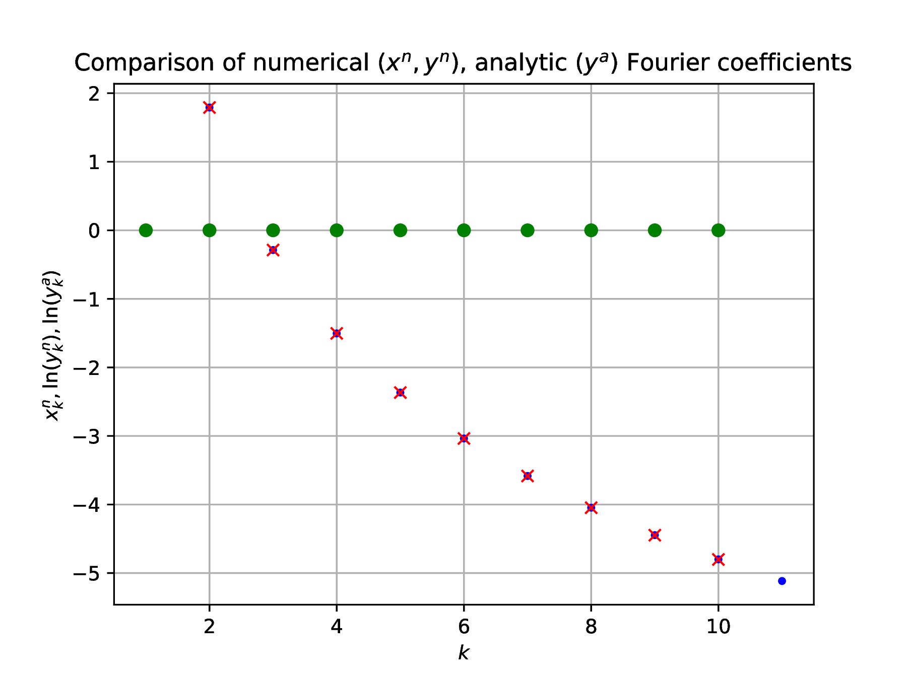
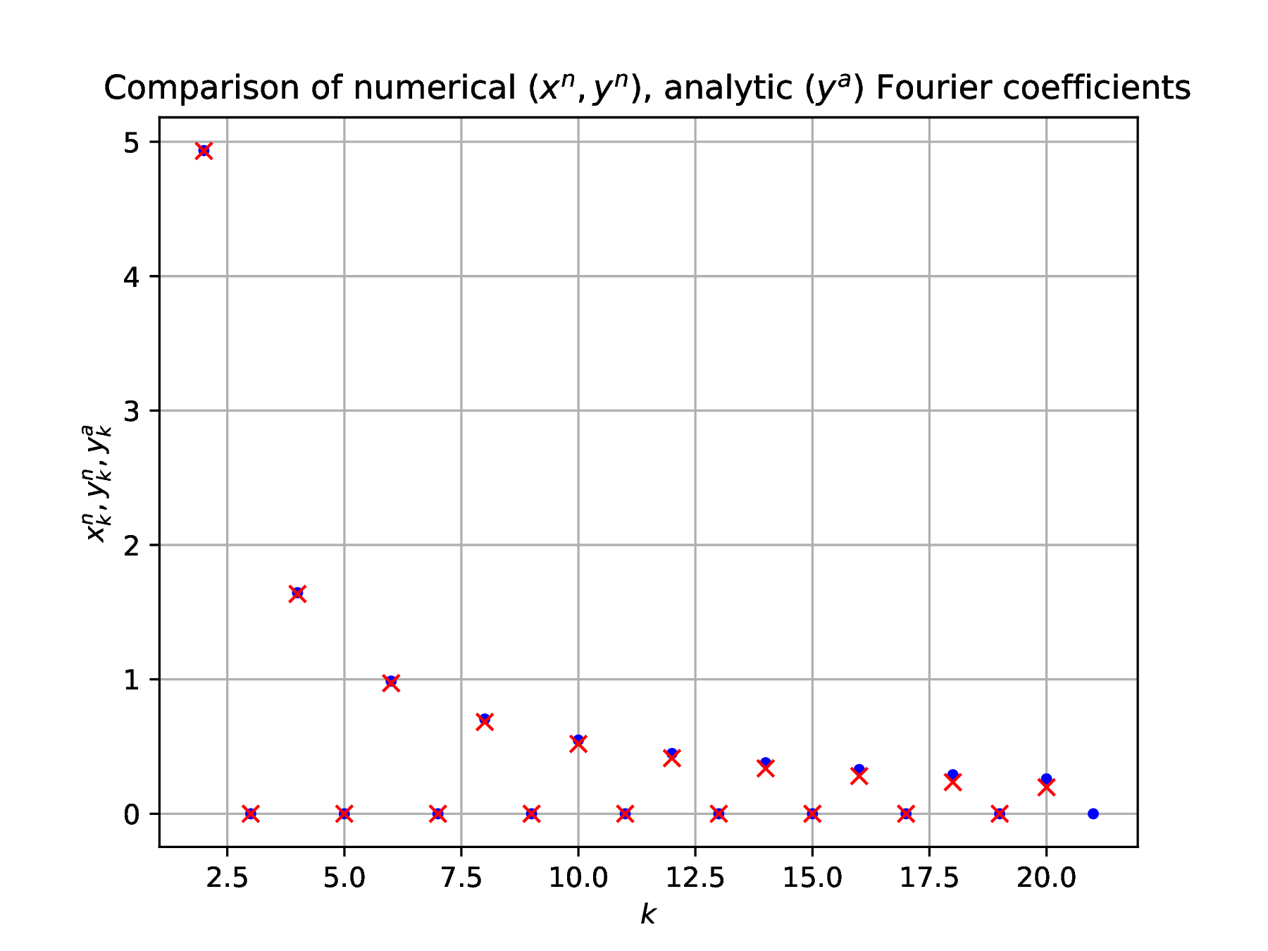
   2. Compare the analytically computed Fourier coefficients with the numerical results obtained in Problem 1, a)-c). Assess the analytically predicted Fourier series convergence by comparison to the numerical results.

      Solution. The relevant basis is case $b$, and numerically computed coefficients are compared against analytical results in Fig. 2 .

      $\circ$

      Figure 2. Numerical $x_k\left(•\right)$, $y_k\left(\times \right)$, recover analytical $x_k=0$, $y_k=12/k^3\left(•\right)$.

      Construct plot

      ∴	m=72; n=10; A,bt = SetUp(m,n,ub,b); coef = A\bt; xn=real(coef); yn=imag(coef);

      ∴	kr = 1:n; yk = 12 ./ kr.^3;

      ∴	clf(); plot(kr,xn,"og",kr.+1,log.(0.5*yk),".b",kr[2:n],log.(yn[2:n]),"xr");

      ∴	xlabel(L"k"); ylabel(L"x_k^n, \ln(y_k^n), \ln(y_k^a)"); grid("on");

      ∴	title(L"Comparison of numerical ($x^n, y^n$), analytic ($y^a$) Fourier coefficients");

      ∴	savefig(homedir()*"/courses/MATH661/homework/H02/Fig2.eps");

      ∴

   3. Carry out series approximations as in Problem 1, a)-d) of

      ${\displaystyle c\left(t\right)=\frac{{\pi }^3}{4}[H\left(t\right)-2H(.t-\pi ).]}$

      where $H\left(x\right)$ is the Heaviside step function

      ${\displaystyle H\left(x\right)=\{\begin{array}{ll}0& x<0\\ 1& x>0\end{array}..}$

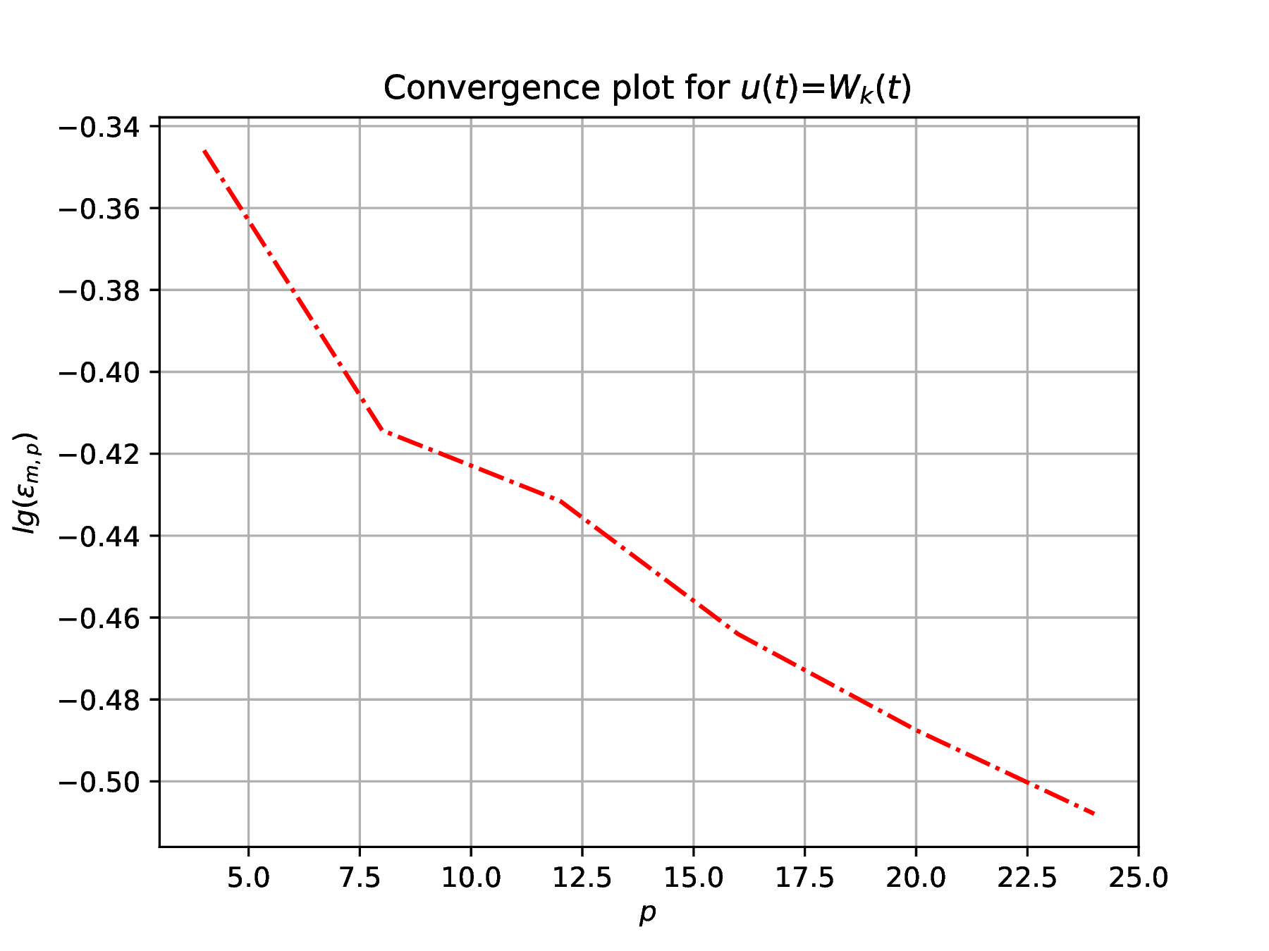
      Solution. The steps of Problem 1 are repeated for $c\left(t\right)$ leading to Fig. 3

      $\circ$Define $H\left(t\right),c\left(t\right)$

      ∴	H(t) = if t<0 return 0; else return 1 end;

      ∴	c(t)=0.25*pi^3*(H(t)-2*H(t-pi));

      ∴

      $\circ$Sample the function $c\left(t\right)$, and construct convergence plots for the four cases

      Note: The benefit from taking the time to code the functions used in Problem 1 is now apparent. Solving problem 2 is immediate: simply change the function that is being approximated.

      ∴	m=100; pr=4:4:24;

      ∴	plotE(m,pr,ua,c,1,"og",L"\cos(k t)","Fig3a");

      ∴	plotE(m,pr,ub,c,2,"xb",L"\exp(-i k t)","Fig3b");

      ∴	plotE(m,pr,uc,c,1,"+k",L"\sin(k t)","Fig3c");

      ∴	plotE(m,pr,ud,c,1,".r",L"W_k(t)","Fig3d");

      ∴

      Figure 3. Comparison of convergence of approximation of $c\left(t\right)$ for different basis sets. Slower convergence is observed by comparison to approximation of $b\left(t\right)$. The fastest convergence is observed for the triangle wave basis $W_k\left(t\right)$.

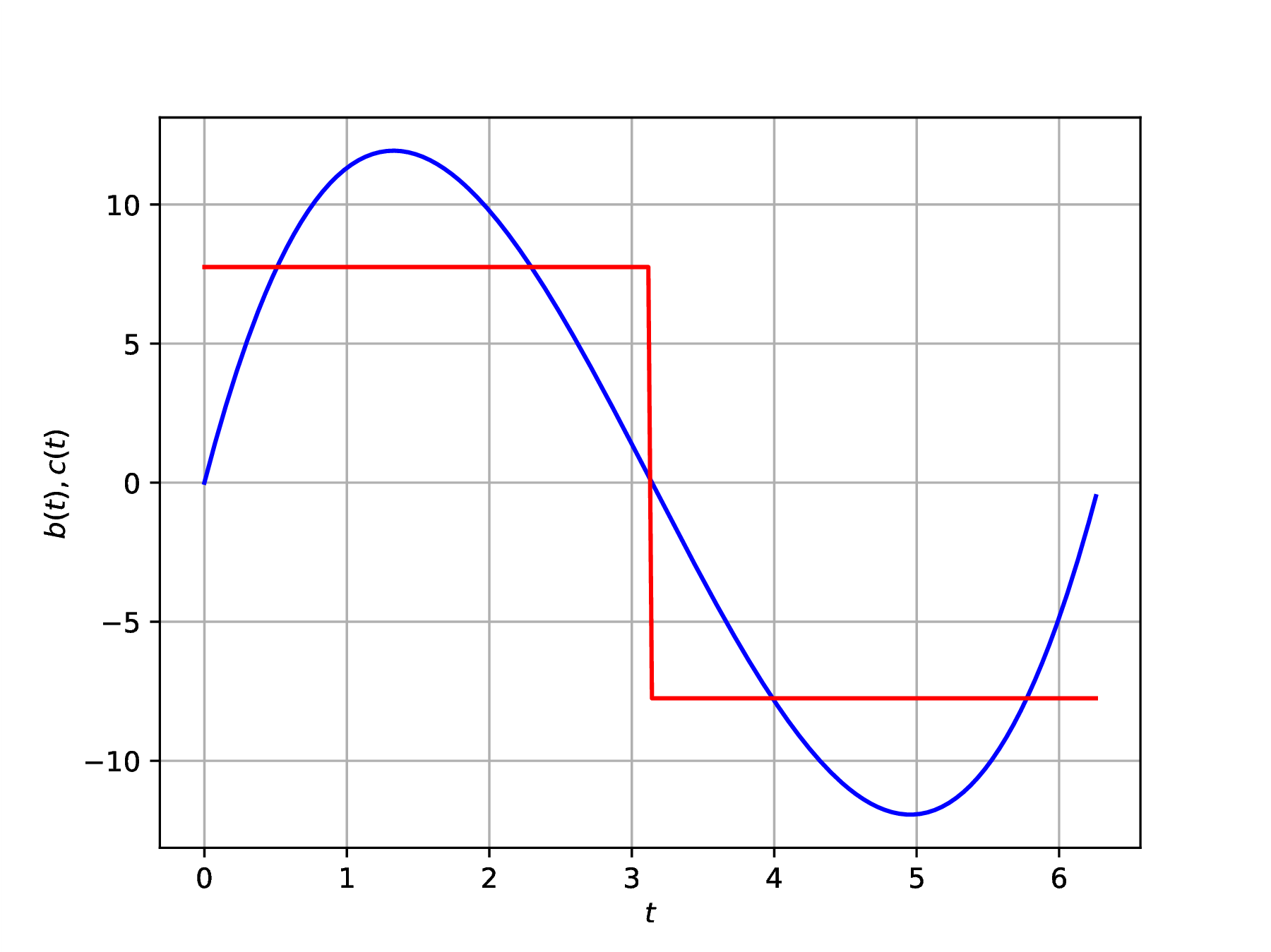
   4. Again, compare analytically evaluated Fourier coefficients with numerical results. How do the approximations of $c\left(t\right)$ behave differently from those of $b\left(t\right)$?

      Solution. Plot $b\left(t\right)$ and $c\left(t\right)$ to gain insight into different behavior (Fig. 4). Note that $c\left(t\right)$ is a discontinuous analogue of $b\left(t\right)$.

      $\circ$

      Figure 4. $b\left(t\right)$ (blue), $c\left(t\right)$ (red)

      ∴	m=250; h=2*pi/m; j=1:m; t=(j.-1).*h; bt=b.(t); ct=c.(t);

      ∴	clf(); plot(t,bt,"-b",t,ct,"-r"); xlabel(L"t"); ylabel(L"b(t), c(t)"); grid("on");

      ∴	savefig(homedir()*"/courses/MATH661/homework/H02/Fig4.eps");

      ∴

      The Fourier coefficients are now

      ${\displaystyle x_k=\frac{1}{\pi }\underset{0}{\overset{2\pi }{\int }}c\left(t\right)\cos (kt)dt=0,y_{2j+1}=\frac{1}{\pi }\underset{0}{\overset{2\pi }{\int }}b\left(t\right)\sin (kt)dt=\frac{{\pi }^2}{2j+1},y_{2j}=0.}$

      $\circ$

      Figure 5. Numerical $y_k\left(\times \right)$, recovers analytical $y_{2j+1}={\pi }^2/(2j+1)\left(•\right)$.

      Construct plot

      ∴	m=72; n=20; A,ct = SetUp(m,n,ub,c); coef = A\ct; xn=real(coef); yn=imag(coef);

      ∴	kr = 1:n; yk = (kr .% 2) .* pi^2 ./ kr;

      ∴	clf(); plot(kr.+1,0.5*yk,".b",kr[2:n],yn[2:n],"xr");

      ∴	xlabel(L"k"); ylabel(L"x_k^n, y_k^n, y_k^a"); grid("on");

      ∴	title(L"Comparison of numerical ($x^n, y^n$), analytic ($y^a$) Fourier coefficients");

      ∴	savefig(homedir()*"/courses/MATH661/homework/H02/Fig5.eps");

      ∴

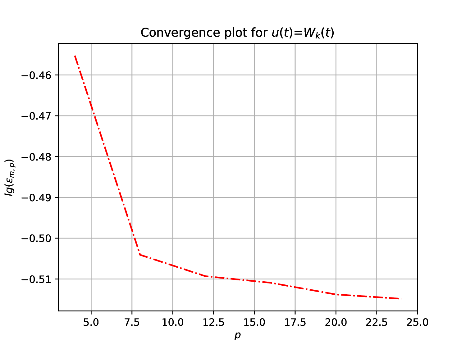
      Convergence is obtained for both $b\left(t\right)$ and $c\left(t\right)$. Convergence is faster for $b\left(t\right)$ in the continuous Fourier basis, while for $c\left(t\right)$ it is faster in the discontinuous triangle wave basis. Convergence is slower for the discontinuous function $c\left(t\right)$ with coefficient decay $\sim 1/k$ by comparison to the coefficient decay $\sim 1/k^3$ for the continuous function $b\left(t\right)$.

Bibliography