 |
|
Posted: 09/13/23
Due: 09/20/23, 11:59PM
Tracks 1 & 2: 1. Track 2: 2.
This homework marks your first foray into realistic scientific computation by applying concepts from linear algebra, specifically using the singular value decomposition to analyze hurricane Lee, still active at this time.
Processing of image data through the tools of linear algebra is often encountered, and in this assignment you shall work with satellite images of hurricane Lee of 2023 Season. Open the following folds and execute the code to set up your environment.
The following commands within a BASH shell brings up an animation of hurricane Lee (ImageMagick package must be installed and in the system path.
The model will use various Julia packages to process image data, carry out linear algebra operations. The following commands build the appropriate Julia environment. The Julia packages are downloaded, compiled and stored in your local Julia library. Note: compiling the Images package takes a long time and it's best to do this within a terminal window. Compiling the packages need only be done once.
Once compiled, packages are imported into the current environment
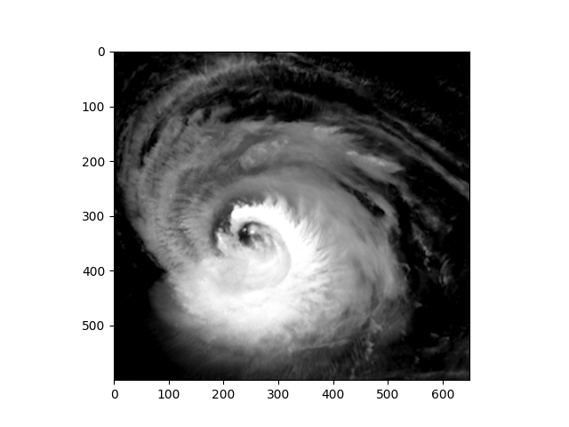
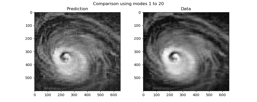
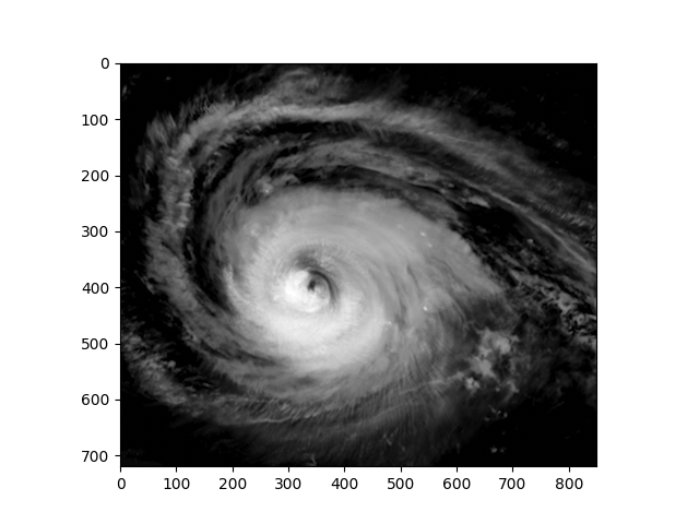
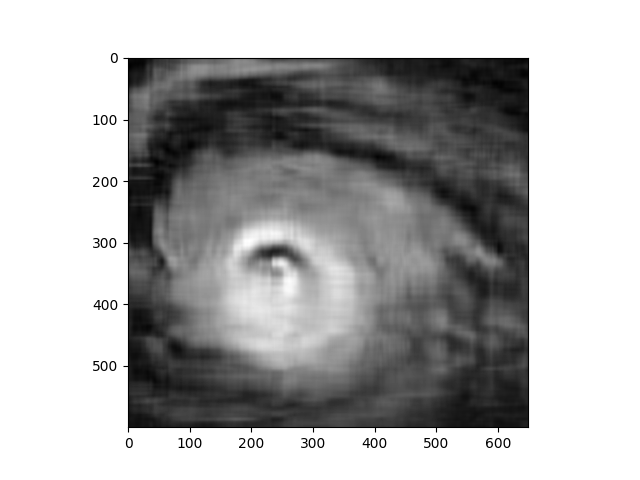
With appropriate packages in place and available, the satellite imagery can be imported into the Julia environment and used to insert images such as the one in Fig. (1).
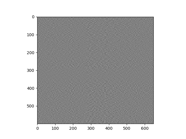
Image data must be quantified, i.e., transformed into numbers prior to analysis. In this case matrices of 32-bit floats are obtained from the gray-scale intensity values associated with each pixel. The 720 by 850 pixel images might be too large for machines with limited hardware resources, so adapt the window to obtain reasonable code execution times, Fig. 2.
|
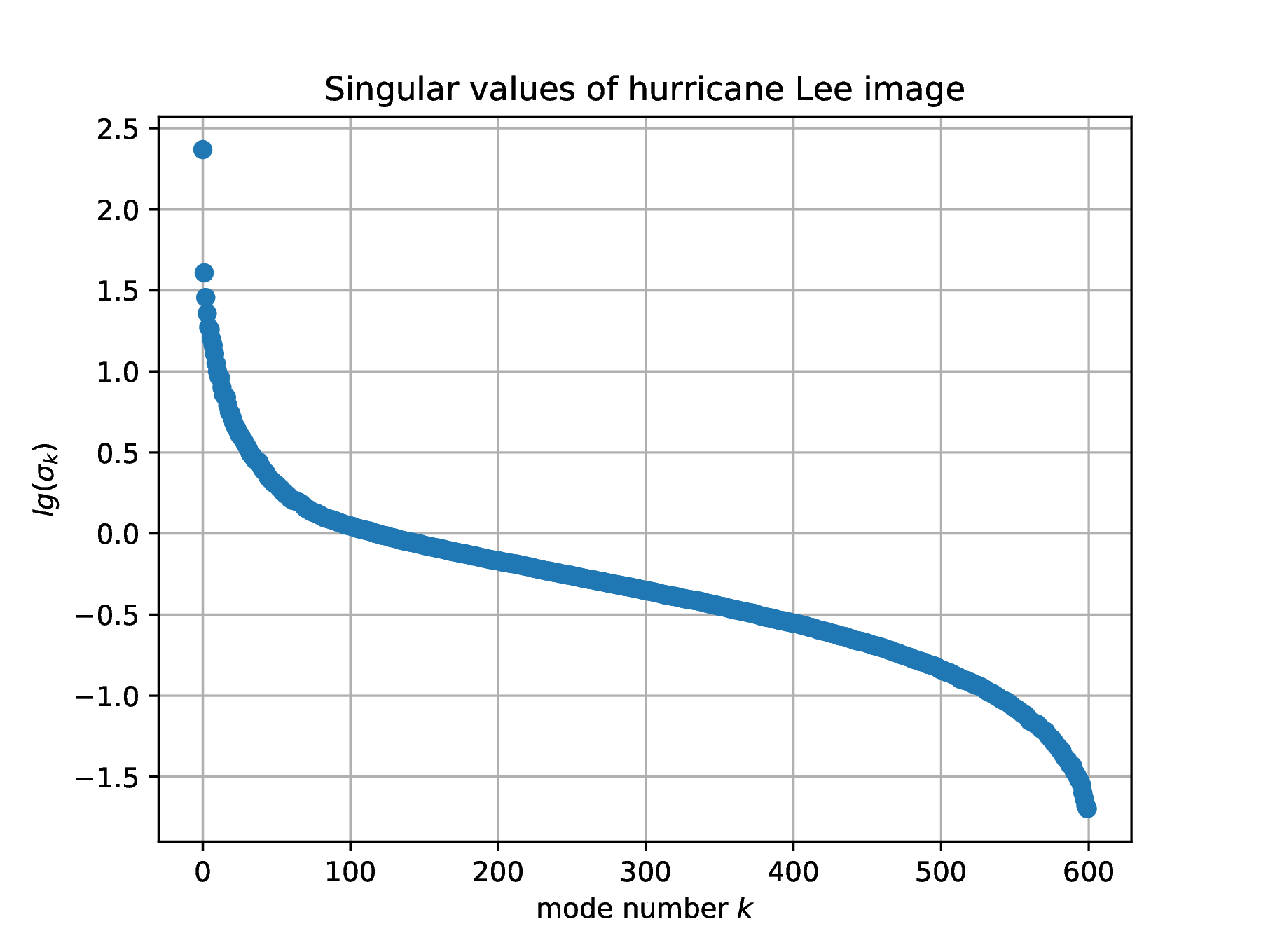
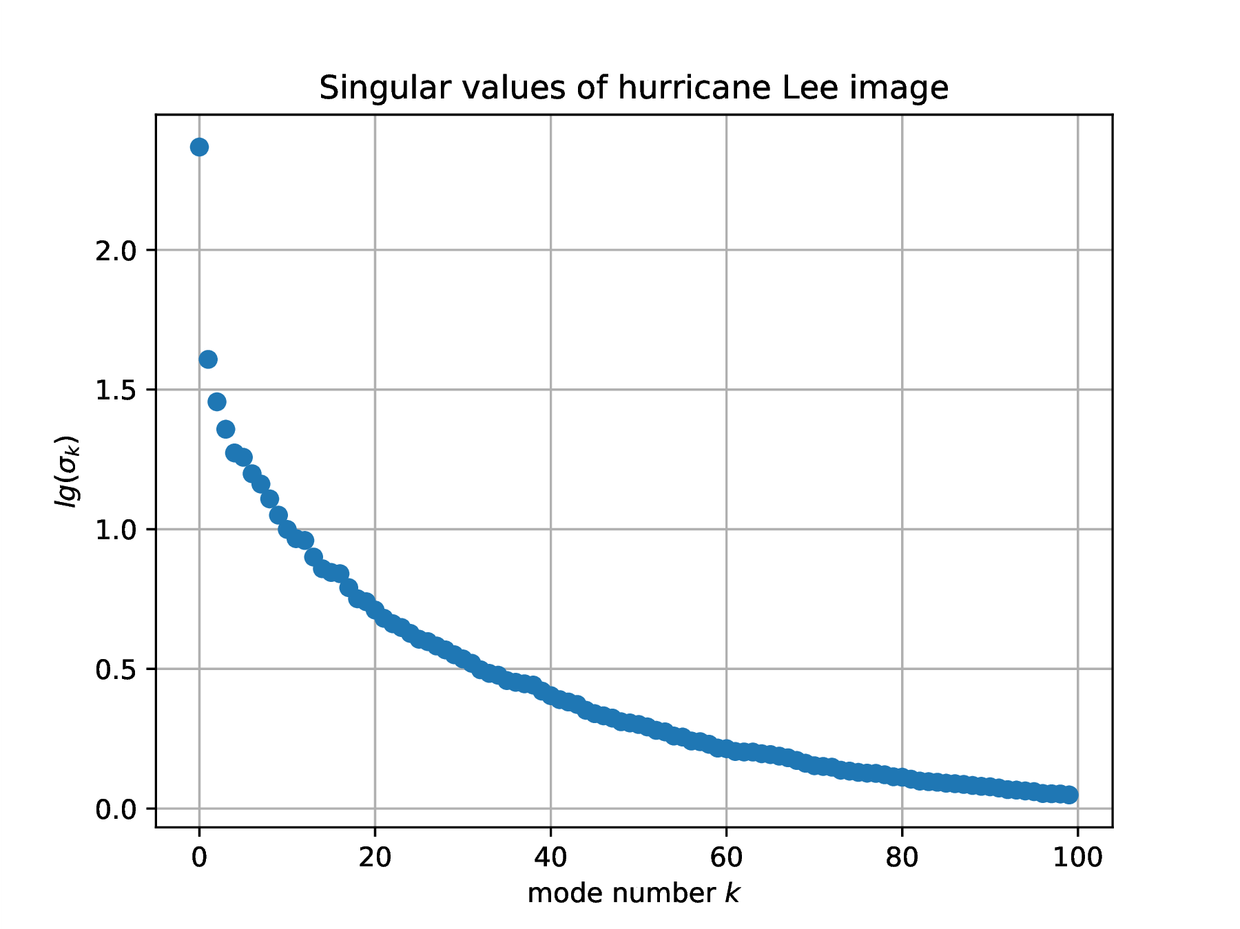
The SVD of the array of floats obtained from an image identifies correlations in gray-level intensity between pixel positions, an encoded description of weather physics. Here are the Julia instructions to compute the SVD of one frame of image data. It is instructive to plot the singular values , in log coordinates.
∴ |
n=32; A=data[:,:,n]; U,S,V=svd(A); |
∴ |
clf(); plot(log10.(S),"o"); xlabel(L"mode number $k$"); ylabel(L"lg(\sigma_k)"); |
∴ |
title("Singular values of hurricane Lee image"); grid("on"); |
∴ |
hwdir=homedir()*"/courses/MATH661/homework/H03"; savefig(hwdir*"/H03Fig03a.eps"); |
∴ |
clf(); plot(log10.(S[1:100]),"o"); xlabel(L"mode number $k$"); ylabel(L"lg(\sigma_k)"); |
∴ |
title("Singular values of hurricane Lee image"); grid("on"); |
∴ |
savefig(hwdir*"/H03Fig03b.eps"); |
∴ |
  |
Define a function rsvd to sum the rank-one updates from to from an SVD,
The sum from to contains the first dominant correlations, identified as large scale weather patterns. The sum from to can be identified as small scale patterns.
  |
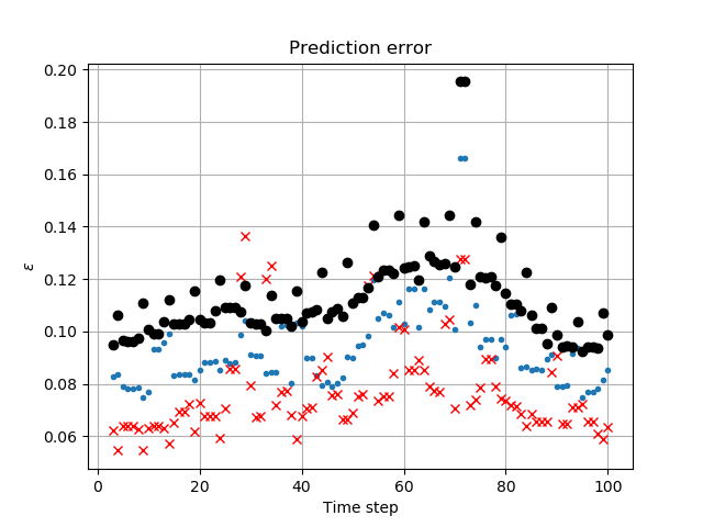
Consider large-scale weather patterns , , obtained from the most significant modes from frames (i.e., different times in the past). Assuming a constant rate of change leads to the prediction
| (3) |
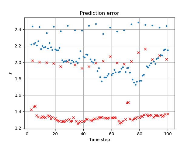
for the known large-scale weather . The prediction error is . Present a plot of the prediction error for various values of over the recorded hurricane data. Analyze your results to answer the question: “can overall storm evolution be predicted by linear extrapolation of past data?”
Define a function to construct prediction at time by linear extrapolation of modes from to at times
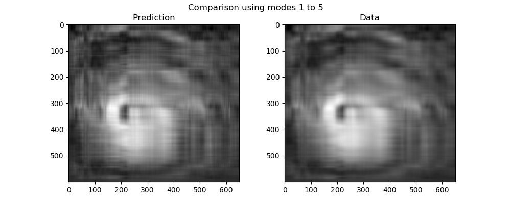
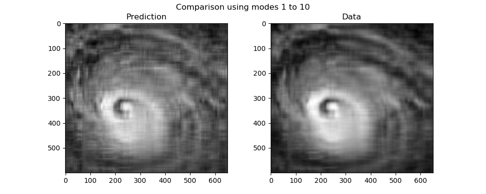
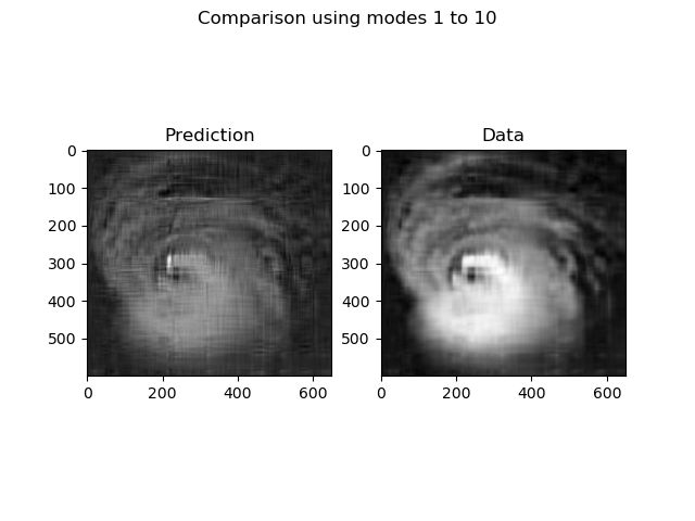
Define a function to compare the coarse grained prediction and data
Define a function to plot the prediction error over the available data
Relative error (Fig. 5) between prediction and observed data increases as with increase in the number of SVD modes (Fig. 6). This might seem surprising at first glance, but the comparison is done on raw data. In almost all real-world applications additional pre/post-processing of data is needed to:
ensure identical illumination in the two images;
align and rotate the images to match overall features (aka “image registration”)
determine whether pixel-by-pixel comparison is meaningful as opposed to derived measures: total cloud cover, position of center, etc.
Bonus point project (4 points). Carry out the above operations. Of particular relevance is the recognition of overall structure in data, in this case the spiral pattern of the anti-cyclone. Think of a way to use this knowledge of the expected overall pattern to better compare predictions to data.
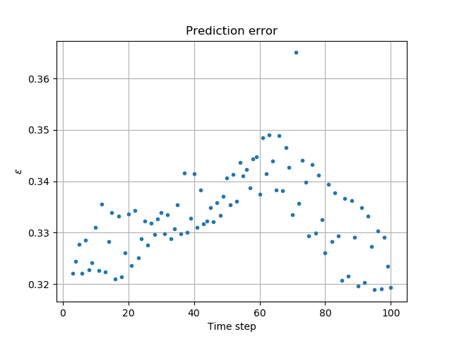
Repeat the above construction of an error plot for local weather patterns for lesser significance modes from to , that lead to prediction
Analyze your results to answer the question: “are small-scale storm features predictable?”
Solution. The key word in the problem statement is “repeat”. Defining purpose-specific functions is not only good coding practice, but saves time in studying similar problems. Here, the previously defined functions are simply invoked with new parameters.
The relative error (Fig. 7) would at first glance indicate no predictive capability of the linear extrapolation of the fine scale structure. However the error definition is inappropriate:
the error measure is global while the modes reflect structure at smaller spatial scales
illumination and registration has not been performed.
As in the previous case, several additional steps have to be carried out on the fine scale data in order to determine whether linear extrapolation is an efficient predictor. In particular, the smaller spatial extent has to be taken into account. A typical processing sequence would:
Ensure equal illumination and registration
Define a window of smaller size, and construct the mean and variance observed when translating the window over the entire image. This would be a data-extracted model of small-scale features of the hurricane
Use observed mean and variance to construct extrapolated small-scale features.
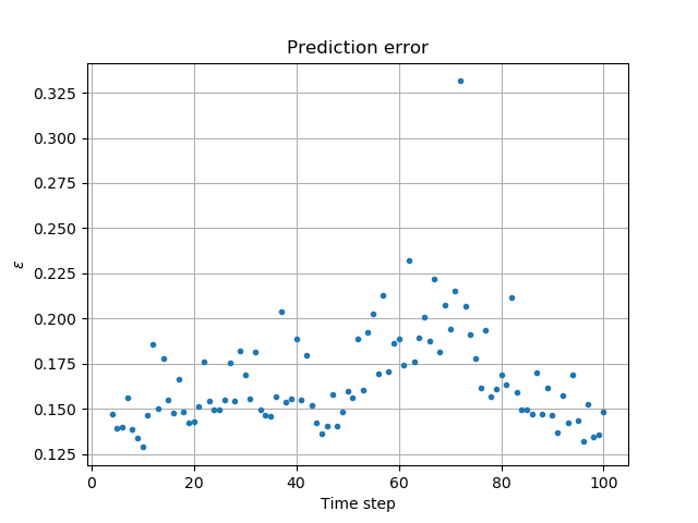
Repeat the above for combined large () and small scale () weather patterns. Experiment with different weights in the linear combination , .
Solution.
Define a function to combine both large and small scales into a weighted average
Define a function to compare the combined large/small-scale prediction and data
Define a function to plot the prediction error over the available data
Formula (3) expresses a degree-one in time prediction
evaluated at . Construct a quadratic prediction based upon data , and compare with degree-one prediction in question 1. Recall that a quadratic can be constructed from knowledge of three points. Again, experiment with various values of .
Solution. Consider with known values at . The quadratic passing through these three points is
and predicts value
hence quadratic predictions are given by
Errors for quadratic extrapolation (Fig. 9) are higher than those for linear extrapolation (Fig. 5). In addition to the errors discussed previously (illumination, registration), higher order extrapolation generally exhibits higher error (to be discussed during presentation of polynomial interpolation).
Use the SVD to investigate how familiar properties for might extend to matrices . For example, on the real axis adding to results in the null element, , so we say is a distance from zero. This easily generalizes to , and the minimal modification of to obtain zero is , , and is distance away from zero. Consider now matrices , with . How far is this matrix from “zero”? By “zero” we shall understand a singular matrix with .
All real numbers can be obtained as the limit of a sequence of rationals , . We say that the rationals is a dense subset of . What about matrix spaces?
Find of minimal norm such that is singular. State how far is from “zero”?
Solution. Seek insight from for which the problem is to find of minimal norm such that . From
deduce that and the solution is . Recall that (the induced 2-norm in the context of an SVD), the maximal amplication factor along any direction within , becomes , interpreted as the amplification factor when . What changes when ? There are now different amplification factors of along different directions. The maximum amplification factor (i.e., the matrix norm) is given by the largest singular value
There is now also a minimal amplification factor, the smallest singular value
The matrix is singular if , stating that along at least one direction the scaling factor is null, , in which case is of minimal norm and trivially satisfies the problem conditions. Assume now that is not singular, , and investigate the smallest amplification factor of , seeking a lower bound for along some arbitrary direction ,
The above states that if then >0 for and is not singular. Hence, in order for to be singular the condition must hold. Use the SVD of and construct
that makes the sum singular, and , the minimal allowed norm.
Prove that any matrix in is the limit of a sequence of matrices of full rank, i.e., the set of full-rank matrices is a dense subset of .
Solution. The SVD of of rank is with . Define sequences such that
Then with are of full rank and .