Posted: 10/18/21

Due: 10/25/21, 11:55PM

1Track 1

1. Determine the interpolating polynomial of

   ${\displaystyle f\left(x\right)=\sin \left(\cos \left(x\right)\right)+\cos \left(\sin \left(x\right)\right)}$

   using $n=2^k$ equidistant nodes in the interval $x\in [-\pi ,\pi ]$, for $k=2,3,4,5$.

   $•$$\circ$Solution. Start by defining a function to sample $f$

   ∴	function sample(n,f,a,b) x=LinRange(a,b,n); y=f.(x) return[x y] end;

   ∴	f(x)=sin(cos(x))+cos(sin(x));

   ∴

   TeXmacs note: Insert->Fold->Folded->Standard is used here to display the above code, but hide the tests of the code.

   Test:

   ∴	xy=sample(3,f,-π,π)

   ${\displaystyle \left[\begin{array}{cc}-3.141592653589793& 0.1585290151921035\\ 0.0& 1.8414709848078965\\ 3.141592653589793& 0.1585290151921035\end{array}\right]}$

   (1)

   ∴	x=xy[:,1]; y=xy[:,2];

   ∴

   $•$$\circ$Gather all interpolation related code into an Interpolation661 module that can be extended and re-used. Iterative editing of the Interpolation661 module is aided by the Revise, InteractiveUtils packages. Add these to your environment through:

   using Pkg; Pkg.add("Revise")

   and place

   using Revise, InteractiveUtils
   ENV["JULIA_EDITOR"]="geany"

   in your TeXmacs tmrepl.jl startup file, or your Julia configuration startup. The last line above sets the editor invoked by the Julia edit() function to be geany.

   TeXmacs note: The code within the Interpolation661 module is included in this document through Insert->Link->Include..., and the insertion can be updated (manually) through Tools->Update->Inclusions. Also define a base directory for saving images.

   ∴	import Pkg

   Busy…

   ∴	dir=homedir()*"/courses/MATH661/images/";

   ∴	Pkg.add(url="/home/student/courses/MATH661/packages/Interpolation661

   module Interpolation661
     
     # Interpolation functions for MATH661.FA.21
     
     export Vandermonde, NewtonBasis
     export Horner, Lagrange, BaryLagrange
     export DivDif, Newton
     
     function Vandermonde(x)
       n=length(x)-1; V=ones(n+1,1)
       for j=1:n
         V = [V x.^j]
       end
       return V
     end
     
     function NewtonBasis(x)
       n=length(x)-1; nj=ones(n+1,1); N=copy(nj)
       for j=1:n
         nj = nj .* (x .- x[j])
         N = [N nj]
       end
       return N
     end
     
     function Horner(t,a)
        n=length(a)-1; p=a[n+1]
        for k=n:-1:1
          p=a[k]+p*t
        end
        return p
     end
     
     function Lagrange(t,x,y)
       n=length(x)-1; p=0
       for i=1:n+1
         w=1
         for j=1:n+1
           if (i!=j) w=w*(t-x[j])/(x[i]-x[j]); end
         end
         p = p + w*y[i]
       end
       return p
     end
     
     function BaryLagrange(t,x,y)
       n=length(x)-1; w=ones(size(x));
       for i=1:n+1
         w[i]=1
         for j=1:n+1
           if (i!=j) w[i]=w[i]/(x[i]-x[j]); end
         end
       end
       q=r=0
       for i=1:n+1
         d=t-x[i]
         if d≈0 return y[i]; end
         s=w[i]/d; q=q+y[i]*s; r=r+s
       end
       return q/r
     end
     
     function DivDif(x,y)
       n=length(x)-1; d=copy(y)
       for i=2:n+1
         for j=n+1:-1:i
           d[j] = (d[j]-d[j-1])/(x[j]-x[j-i+1])
         end
       end
       return d
     end
     
     function Newton(t,x,d)
       n=length(x)-1; p=d[1]; r=1
       for k=2:n+1
         r = r*(t-x[k-1])
         p = p + d[k]*r
       end
       return p
     end
     
     function Bspline(t,x,k)
       n=length(x); m=length(t); B=zeros(m,n)
       B[:,j]
     end
     
   end
     
   

   In each case:

   1. Find the coefficients in the monomial basis by solving the system $𝑽𝒂=𝒚$, where $y_i=f\left(x_i\right)$. Use the Julia backslash operator.

      Solution. Allocate space to store the $𝒂$ coefficients for all $k$

      ∴	kmn=2; kmx=5; kr=2:5; nRows=2^kmx; nCols=kmx-kmn+1;

      ∴	a=zeros(nRows,nCols);

      ∴

      Define a function to sample $f:[-\pi ,\pi ]\to ℝ$-, the Vandermonde matrix, and determine $𝒂$

      ∴	function aCalc(f,n) xy = sample(n,f,-π,π); x = xy[:,1]; y = xy[:,2] V = Vandermonde(x); a = V \ y end;

      ∴

      Invoke the function in a loop over the $k$-range, and plot the log and sign of the coefficients

      ∴	figure(1); clf(); a=zeros(nRows,nCols);

      ∴	for k in kr n = 2^k; j=k-kmn+1; nr=1:n; lnr=log10.(nr).+1 a[1:n,j] = aCalc(f,n) subplot(3,1,1); plot(nr,log10.(abs.(a[1:n,j])),"o--") subplot(3,1,2); plot(lnr,log10.(abs.(a[1:n,j])),"o--") subplot(3,1,3); plot(1:n,sign.(a[1:n,j]),"o--") end;

      ∴	subplot(3,1,1); xlabel("i"); ylabel("lg|a[i]|"); grid("on")

      ∴	title("Monomial basis coefficients");

      ∴	subplot(3,1,2); xlabel("lg(i)"); ylabel("sgn(a[i])"); grid("on")

      ∴	subplot(3,1,3); xlabel("i"); ylabel("sgn(a[i])"); grid("on")

      ∴	savefig(dir*"S06Fig01.eps");

      ∴

      Figure 1. Note the overall decay of the monomial basis coefficients in absolute value, an indication of a converging approximation. However, the rate of convergence is slow

   2. Find the coefficients in the Newton basis by solving the system $𝑵𝒄=𝒚$. Use the Julia backslash operator.

      Solution. As above, define a function to form the Newton basis and solve the resulting system.

      ∴	function cCalc(f,n) xy = sample(n,f,-π,π); x = xy[:,1]; y = xy[:,2] N = NewtonBasis(x); c = N \ y end;

      ∴

      Invoke the function in a loop over the $k$-range, and plot the log of coefficients

      ∴	figure(1); clf(); c=zeros(nRows,nCols);

      ∴	for k in kr n = 2^k; j=k-kmn+1; nr=1:n; lnr=log10.(nr).+1 c[1:n,j] = cCalc(f,n) subplot(3,1,1); plot(nr,log10.(abs.(c[1:n,j])),"o--") subplot(3,1,2); plot(lnr,log10.(abs.(c[1:n,j])),"o--") subplot(3,1,3); plot(1:n,sign.(c[1:n,j]),"o--") end;

      ∴	subplot(3,1,1); xlabel("i"); ylabel("lg|a[i]|"); grid("on")

      ∴	title("Newton basis coefficients");

      ∴	subplot(3,1,2); xlabel("lg(i)"); ylabel("sgn(a[i])"); grid("on")

      ∴	subplot(3,1,3); xlabel("i"); ylabel("sgn(a[i])"); grid("on")

      ∴	savefig(dir*"S06Fig02.eps");

      ∴

      Figure 2. Comparison of monomial and Newton basis coefficients.

   3. Find the coefficients in the Newton basis by computing the table of divided differences.

      Solution. The diagonal of the divided difference table are the coefficients in the Newton basis computed above. Apply DivDif from the Interpolation661 module and compare.

      ∴	d=zeros(nRows,nCols);

      ∴	for k in kr n = 2^k; j=k-kmn+1 xy = sample(n,f,-π,π); x = xy[:,1]; y = xy[:,2] d[1:n,j] = DivDif(x,y) err = norm(d[1:n,j]-c[1:n,j]) @printf("k=%d n=%d err=%6.3e\n",k,n,err); end;

      k=2 n=4 err=1.734e-17

      k=3 n=8 err=1.006e-16

      k=4 n=16 err=1.011e-15

      k=5 n=32 err=1.457e-14

      ∴

      In all cases the results are identical to within machine precision

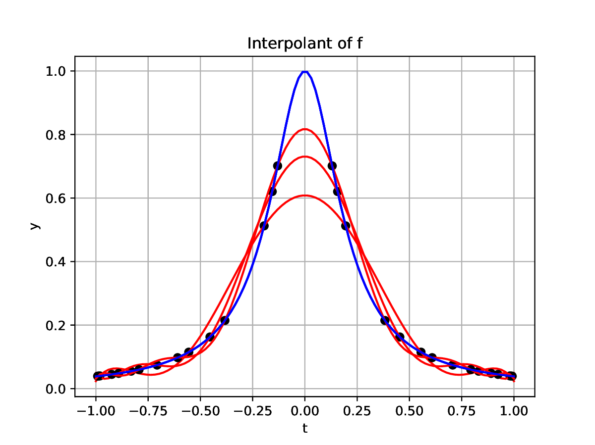
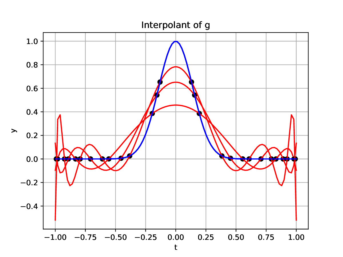
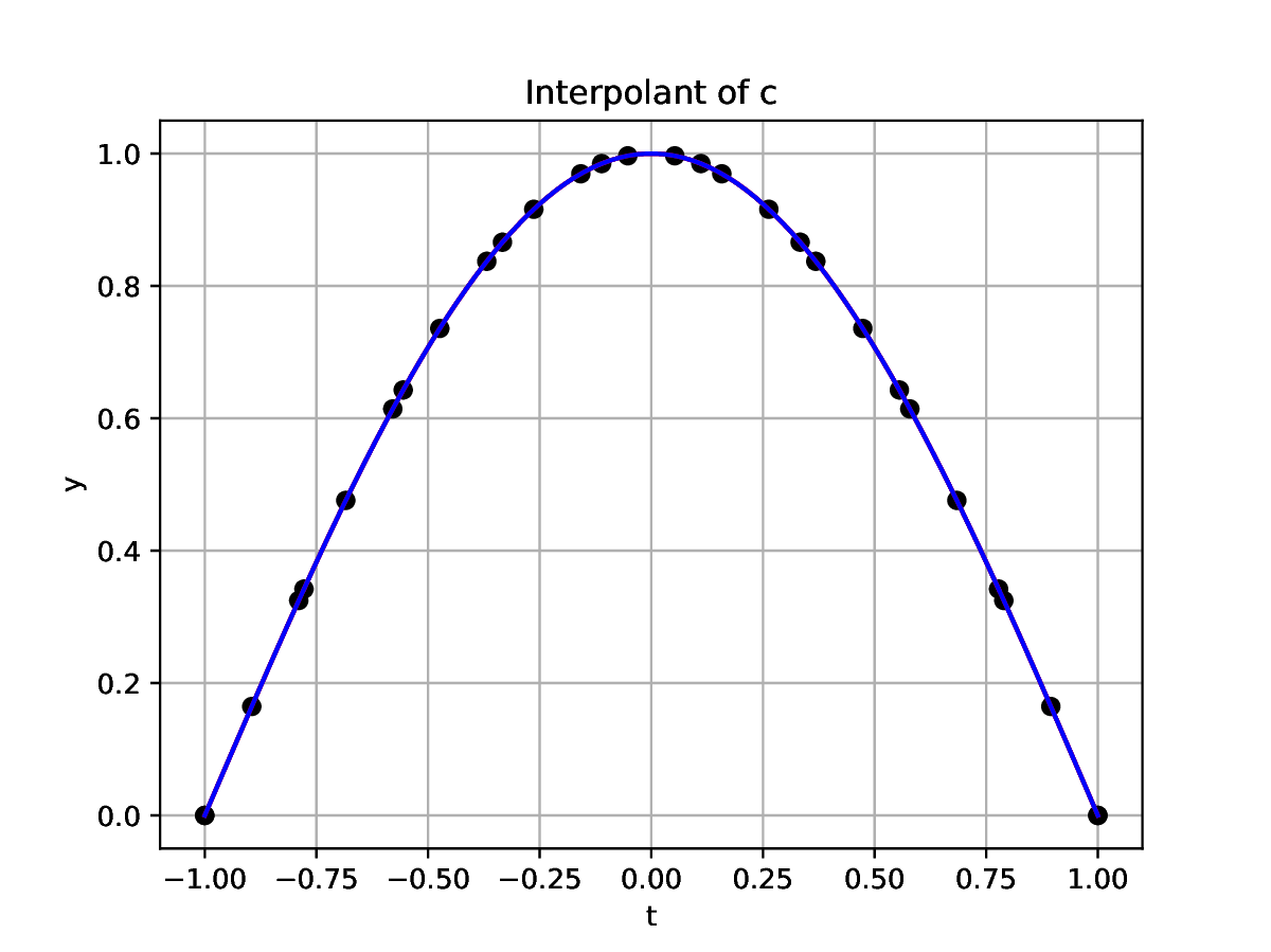
   4. Plot the above approximations evaluated at $n=2^6$ equidistant points along with the plot of the exact function $f\left(x\right)$. Comment on what you observe.

      Solution. The values of the monomial and Newton forms of the interpolant are obtained by Horner's scheme for each basis set

      ∴	figure(1); clf(); n=2^6;

      ∴	ty=sample(n,f,-π,π); t=ty[:,1]; y=ty[:,2];

      ∴	subplot(1,2,1); plot(t,y); plot(t[1:2:n],y[1:2:n],"o");

      ∴	for k in kr j=k-kmn+1; local n=2^k; yN = Horner.(t,Ref(a[1:n,j])) plot(t,yN) end

      ∴	xlabel("t"); ylabel("p(t)"); title("Monomial interpolants");

      ∴	grid("on");

      ∴	subplot(1,2,2); plot(t,y); plot(t[1:2:n],y[1:2:n],"o");

      ∴	for k in kr j=k-kmn+1; local n=2^k; local x=LinRange(-π,π,n) yN = Newton.(t,Ref(x),Ref(d[1:n,j])) plot(t,yN) end

      ∴	xlabel("t"); ylabel("p(t)"); title("Newton interpolants");

      ∴	grid("on");

      ∴	savefig(dir*"S06Fig03.eps");

      Figure 3. Monomial and Newton forms of the interpolant of $f$ evaluated at finer sampling. Small errors arise only near endpoints.

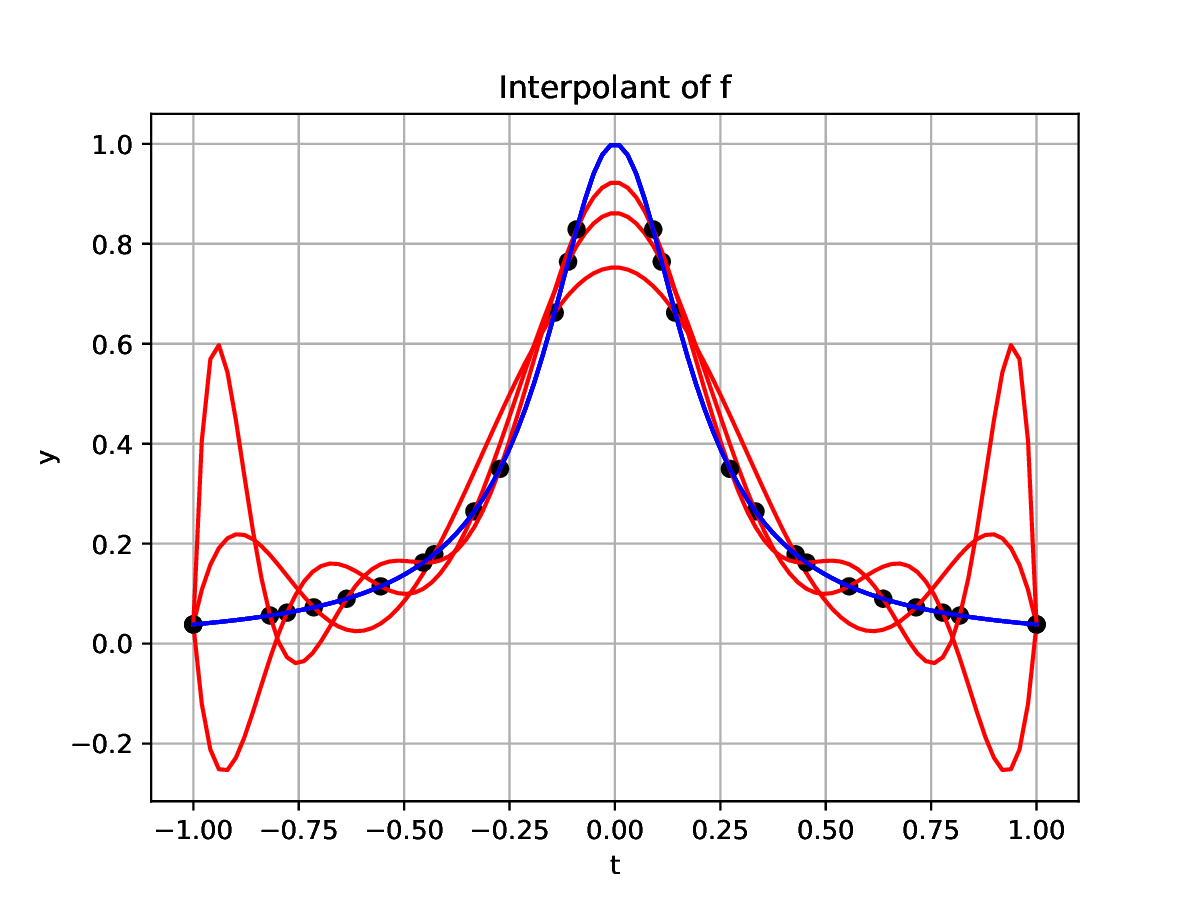
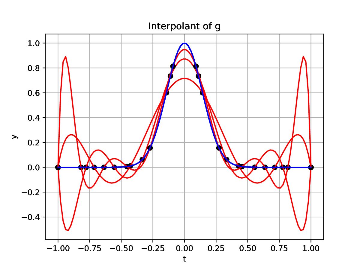
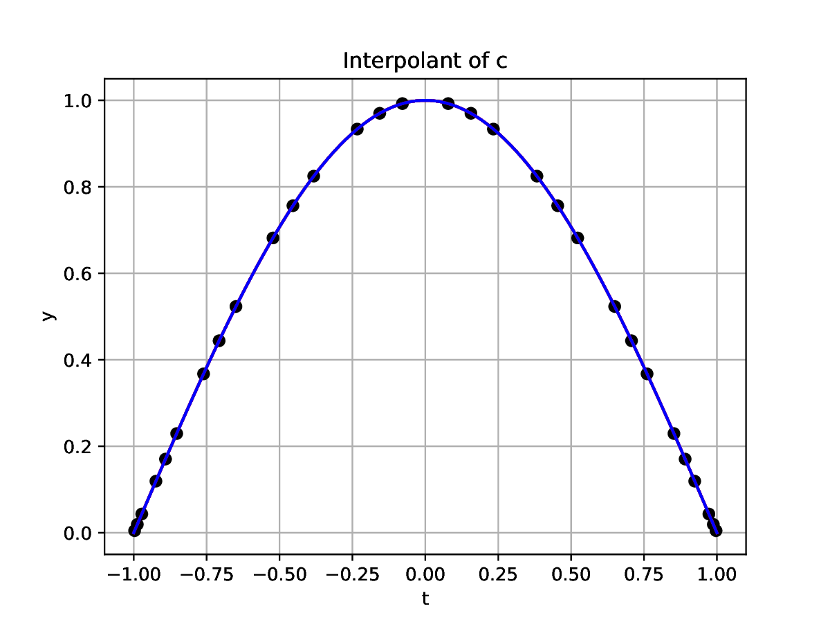
2. Revisit the approximation of the Runge function from HW03. Comment on the accuracy of polynomial approximation of the Runge function by comparison to that of $f\left(x\right)$.

   Solution.

   ∴	figure(1); clf(); n=2^6; Runge(t) = 1/(1+25*t^2);

   ∴	ty=sample(n,f,-π,π); t=ty[:,1]; y=ty[:,2];

   ∴	subplot(1,2,1); plot(t,y); plot(t[1:2:n],y[1:2:n],"o");

   ∴	for k in kr j=k-kmn+1; local n=2^k; yN = Horner.(t,Ref(a[1:n,j])) plot(t,yN) end

   ∴	xlabel("t"); ylabel("p(t)"); title("Interpolant of f");

   ∴	grid("on");

   ∴	subplot(1,2,2); ty=sample(n,Runge,-π,π); t=ty[:,1]; y=ty[:,2]; plot(t,y); plot(t[1:2:n],y[1:2:n],"o");

   ∴	for k in kr j=k-kmn+1; local n=2^k aR = aCalc(Runge,n) yR = Horner.(t,Ref(aR)) plot(t,yR) end

   ∴	xlabel("t"); ylabel("p(t)"); title("Interpolant of Runge function");

   ∴	grid("on");

   ∴	savefig(dir*"S06Fig04.eps");

   Figure 4. Comparison of interpolants of $f$ and Runge function based on equidistant sampling. The interpolation of $f$ is convergent, that of the Runge function is not, with large errors at end points.

2Track 2

1. Read “Barycentric Lagrange Interpolation” in SIAM Review, 2004 Vol. 46, No. 3, pp. 501–517 by Jean-Paul Berrut and Lloyd N. Trefethen.

2. Implement functions to construct the divided-difference coefficients of the Newton interpolating polynomial, and evaluate the resulting polynomial for arbitrary $x$. Test on $f\left(x\right)$ from Track 1, Q1.

   Solution. See above and Interpolation661 module

3. Implement functions to construct the barycentric Lagrange formulas (3.3), (4.2), and test on $f\left(x\right)$.

   Solution. Using BaryLagrange from Interpolation661 module:

   ∴	figure(1); clf(); n=2^6;

   ∴	ty=sample(n,f,-π,π); t=ty[:,1]; y=ty[:,2];

   ∴	plot(t,y); plot(t[1:2:n],y[1:2:n],"o");

   ∴	for k in kr j=k-kmn+1; local n=2^k; xy = sample(n,f,-π,π); x = xy[:,1]; local y = xy[:,2] yB = BaryLagrange.(t,Ref(x),Ref(y)) plot(t,yB) end

   ∴	xlabel("t"); ylabel("p(t)"); title("Barycentric Lagrange interpolant");

   ∴	grid("on");

   ∴	savefig(dir*"S06Fig05.eps");

   ∴

   Figure 5. Barycentric Lagrange interpolants of $f$ evaluated on finer division. The approximations are convergent with small errors at end points.