MATH661 HW06 - Interpolation

MATH661 HW06 - Interpolation

Posted: 10/11/23

Due: 10/18/23, 11:59PM

Beginning with this assignment, homework tasks are described at a higher level. Apply your experience from previous assignments to cogently formulate a solution.

1Track 1 & 2

Study the convergence of polynomial interpolation, $p_{n} (x_{i}) = f (x_{i})$ , $i = 1, 2, \dots, n$ with increasing number of sample points $n$ for the following functions:

$f : [- 1, 1] \to ℝ$ , $f (t) = \cos (π t / 2)$ ;
$f : [- 1, 1] \to ℝ$ , $f (t) = 1 / (1 + 25 t^{2})$ ;
$f : [- 1, 1] \to ℝ$ , $f (t) = \exp (- 25 t^{2})$ .

For each case consider both equidistant and Chebyshev sample points, present plots of the function and interpolant, plots of the error as a function of $n$ , and compare the observed error with that predicted by the formula

e (t) = f (t) - p (t) = \frac{f^{(n + 1)} (ξ_{t})}{(n + 1)!} \prod_{i = 0}^{n} (t - x_{i}) .

Comment on what you observe.

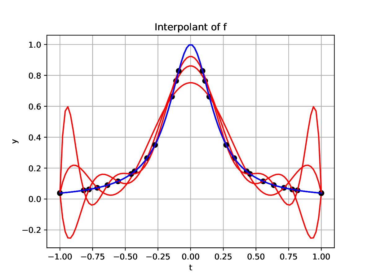
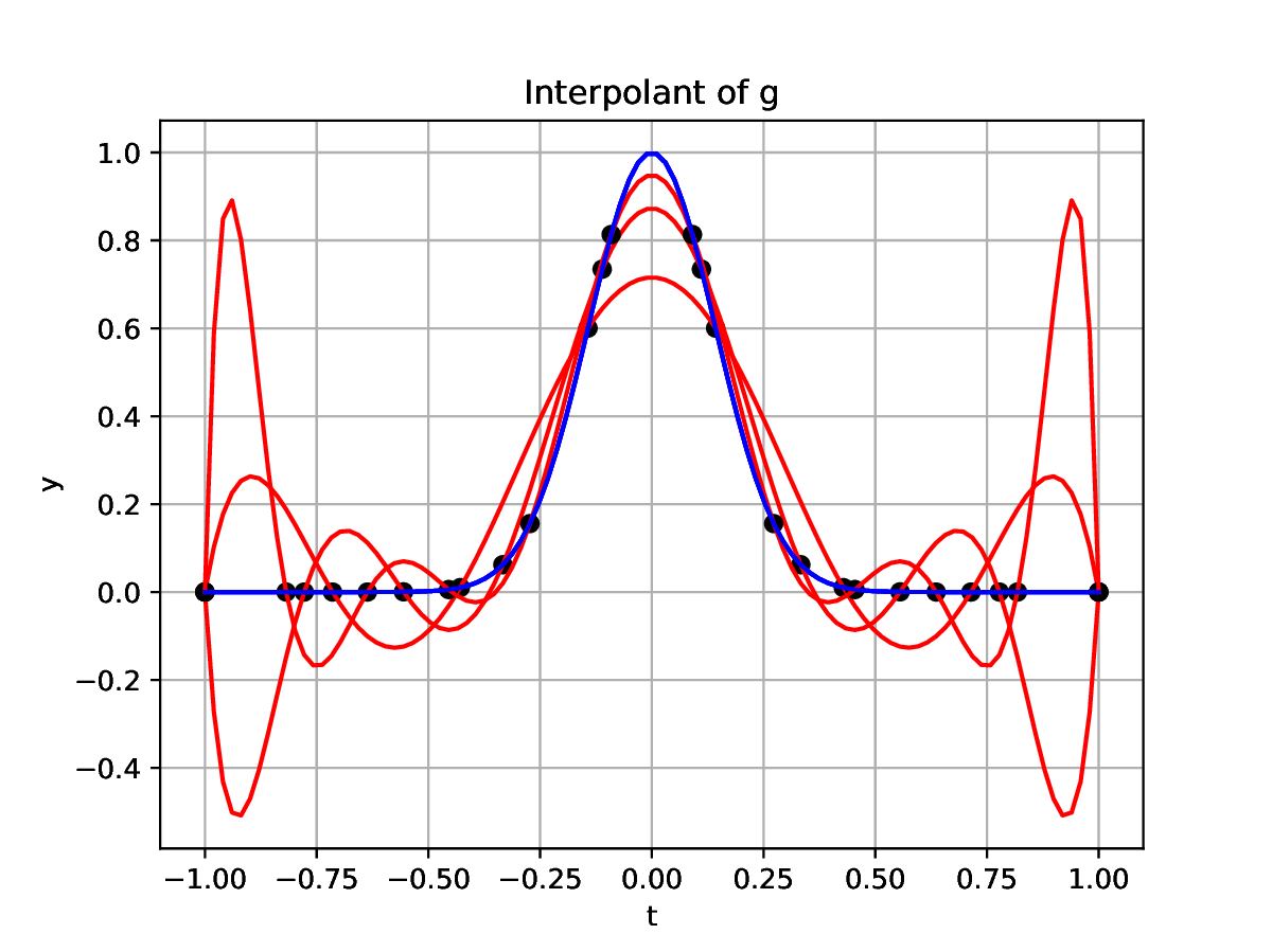
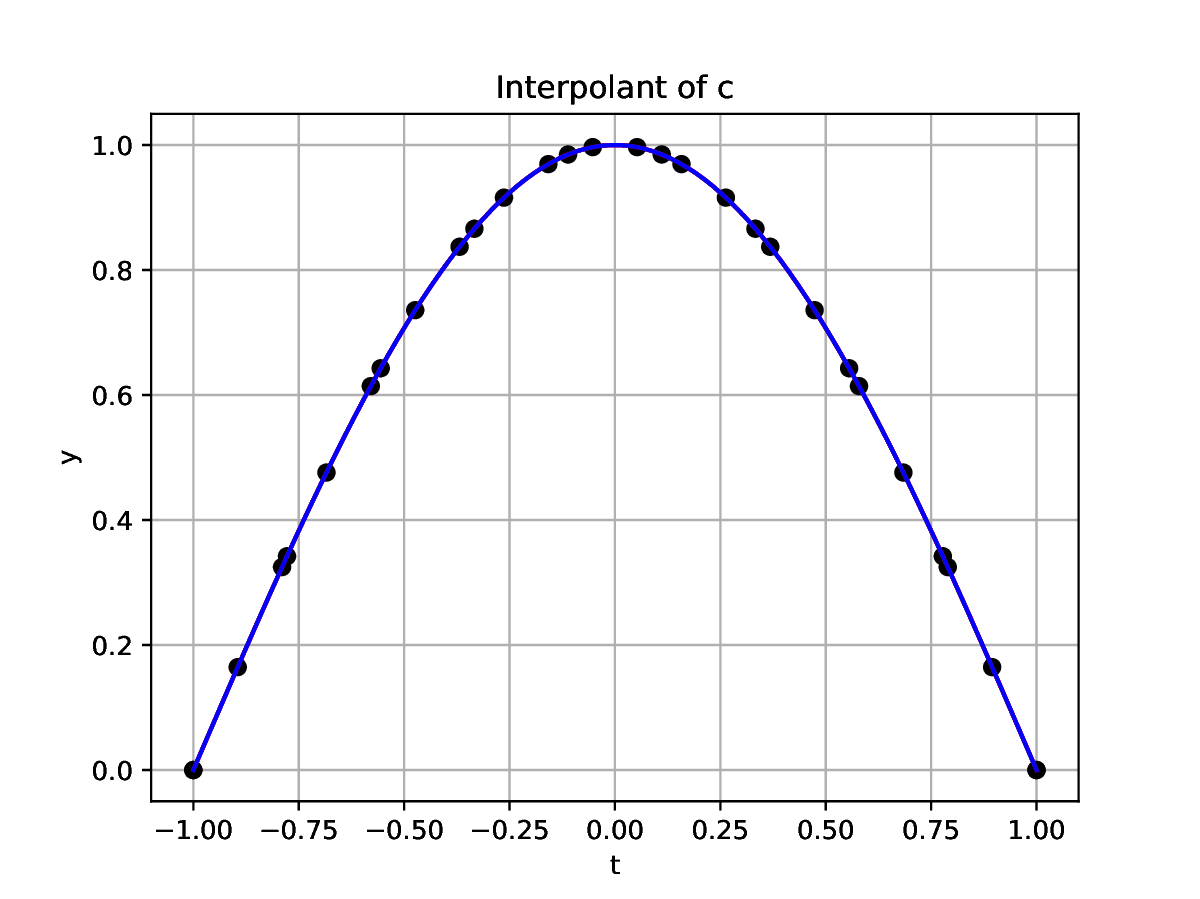
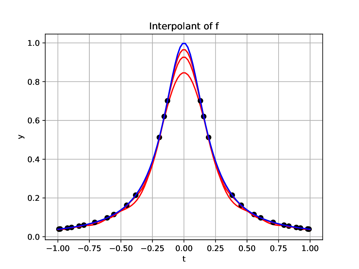
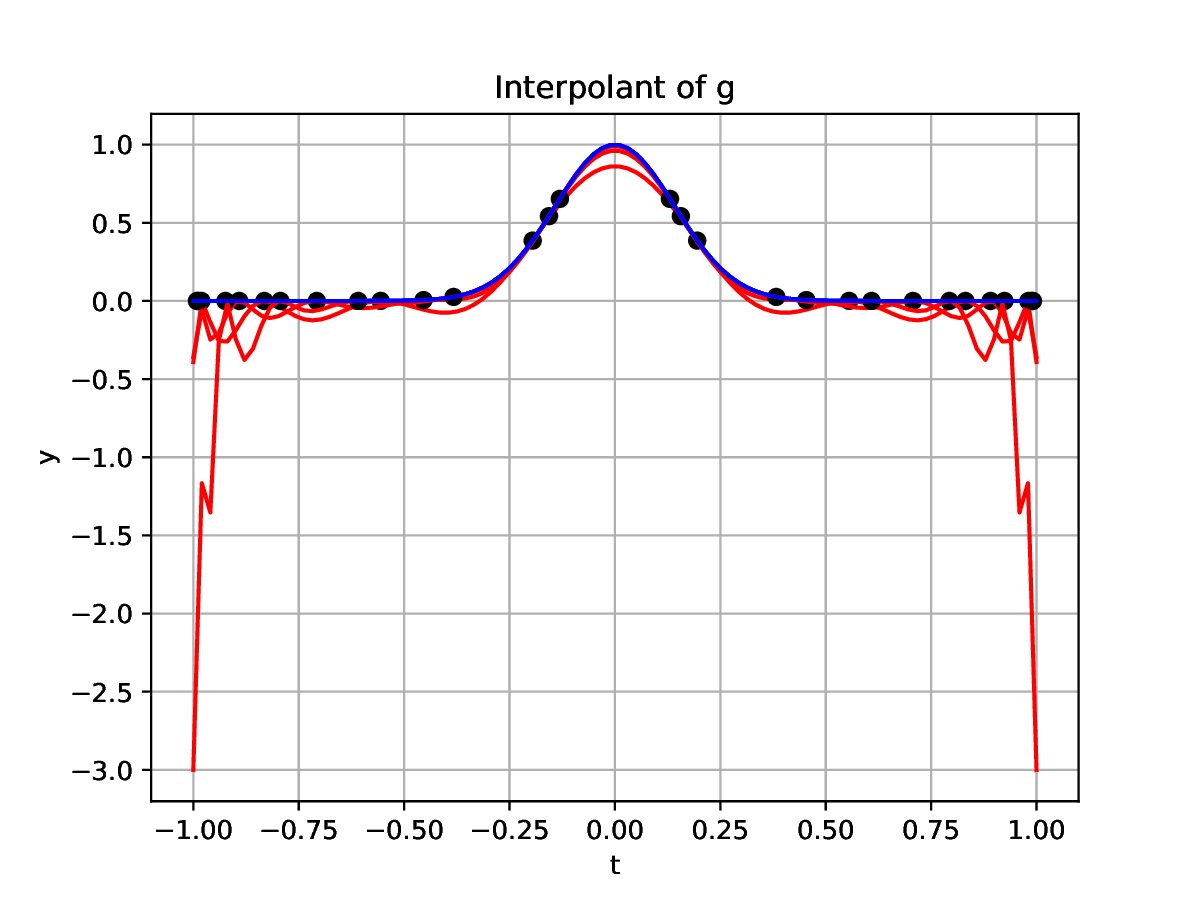
Solution. Use functions from L19 to obtain results in Fig. 1.

$\circ$

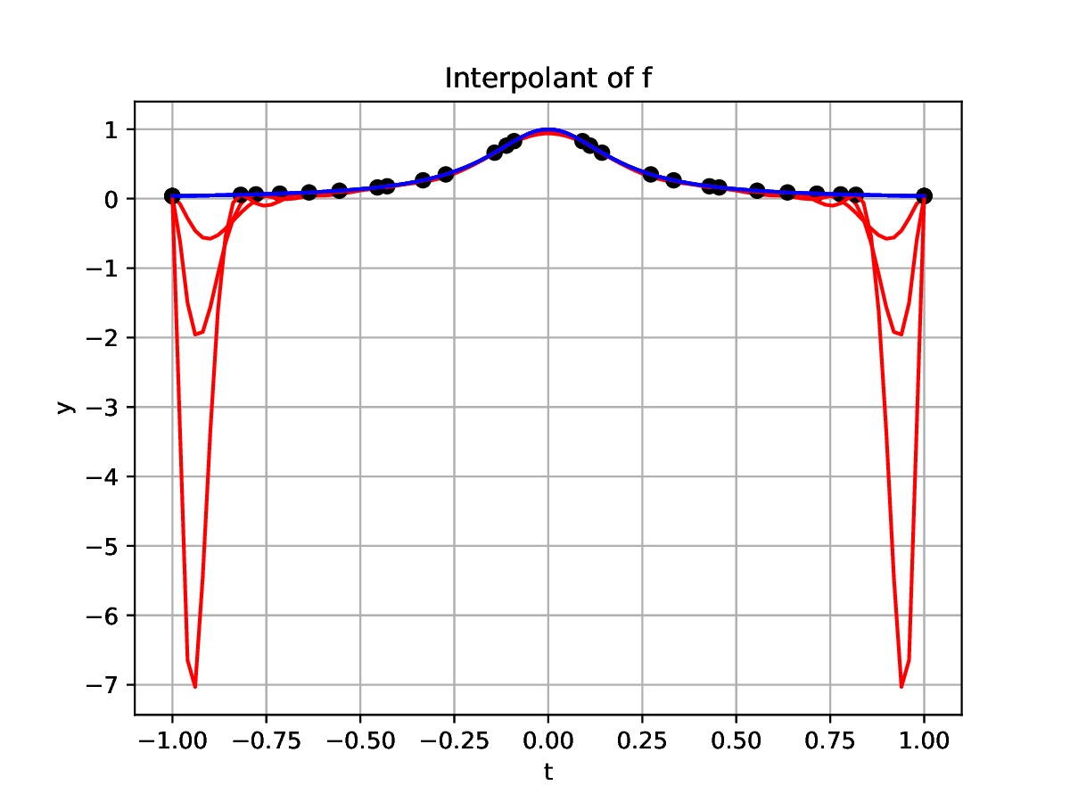
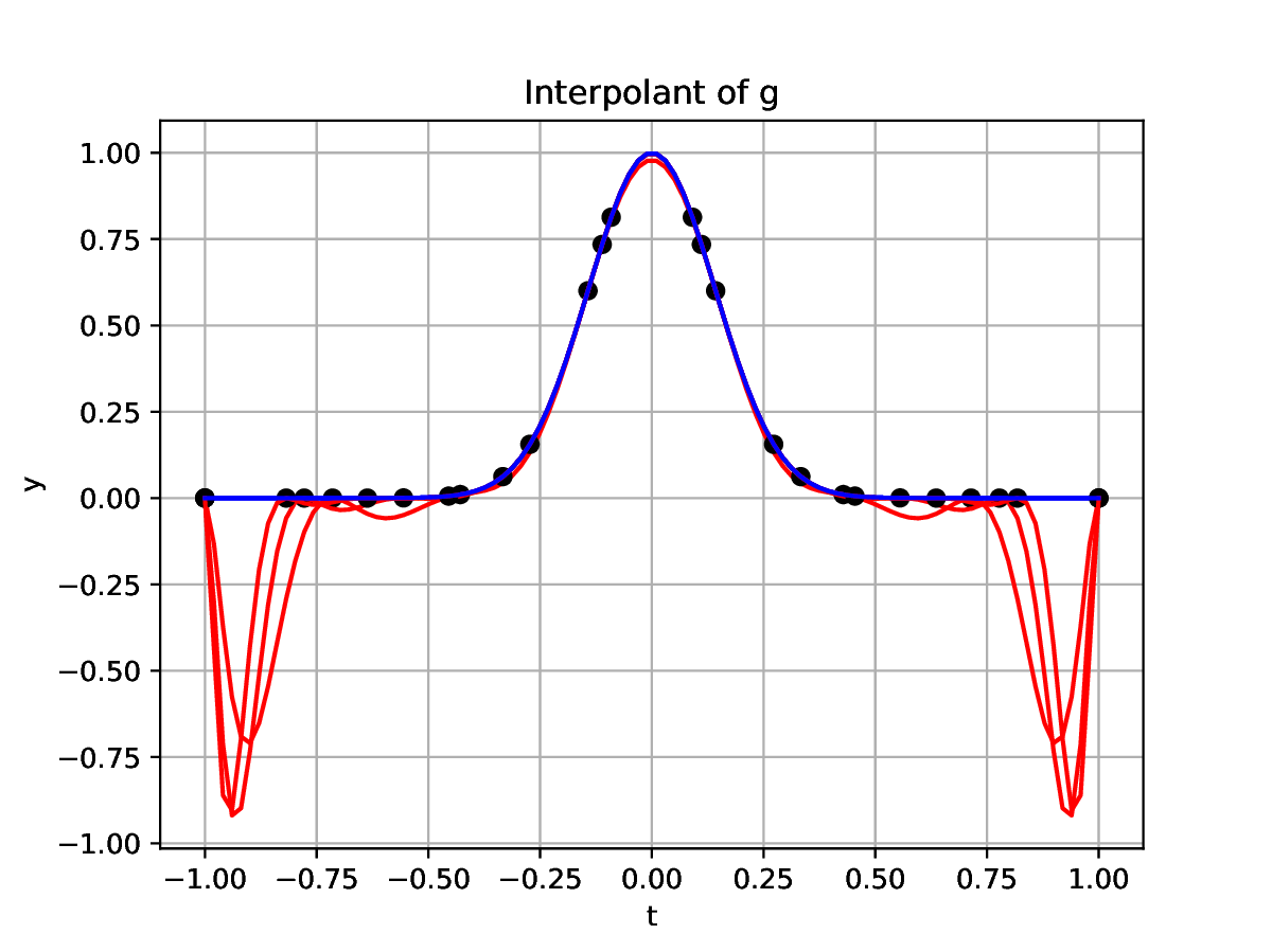
Figure 1. Interpolation results for equidistant partitions of $f (t) \in {\cos (π t / 2), 1 / (1 + 25 t^{2}), \exp (- 25 t^{2})}$

∴	function MonomialBasis(t,n) m=size(t)[1]; A=ones(m,1); for j=1:n-1 A = [A t.^j] end return A end;

∴

function plotInterp(a,b,f,Basis,m,n,M,txt)
  data=sample(a,b,f,m); t=data[1]; y=data[2]
  Data=sample(a,b,f,M); T=Data[1]; Y=Data[2]
  A = Basis(t,n); c = A\y; z = Basis(T,n)*c
  plot(t,y,"ok",T,z,"-r",T,Y,"-b"); grid("on");
  xlabel("t"); ylabel("y");
  title(txt)
end;

∴	function sample(a,b,f,m) t = LinRange(a,b,m); y = f.(t) return t,y end;

∴	c(t)=cos(pit/2); f(t)=1/(1+25t^2); g(t)=exp(-(5*t)^2);

∴	FigPrefix=homedir()*"/courses/MATH661/homework/H06/";

∴	clf(); plotInterp(-1,1,c,MonomialBasis,10,10,100,"Interpolant of c");

∴	plotInterp(-1,1,c,MonomialBasis,20,20,100,"Interpolant of c");

∴	savefig(FigPrefix*"Fig01a.eps")

∴	clf(); plotInterp(-1,1,f,MonomialBasis,8,8,100,"Interpolant of f");

∴	plotInterp(-1,1,f,MonomialBasis,10,10,100,"Interpolant of f");

∴	plotInterp(-1,1,f,MonomialBasis,12,12,100,"Interpolant of f");

∴	savefig(FigPrefix*"Fig01b.eps")

∴	clf(); plotInterp(-1,1,g,MonomialBasis,8,8,100,"Interpolant of g");

∴	plotInterp(-1,1,g,MonomialBasis,10,10,100,"Interpolant of g");

∴	plotInterp(-1,1,g,MonomialBasis,12,12,100,"Interpolant of g");

∴	savefig(FigPrefix*"Fig01c.eps")

∴

$\circ$

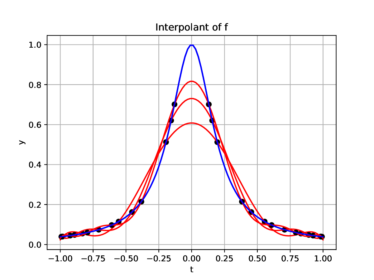
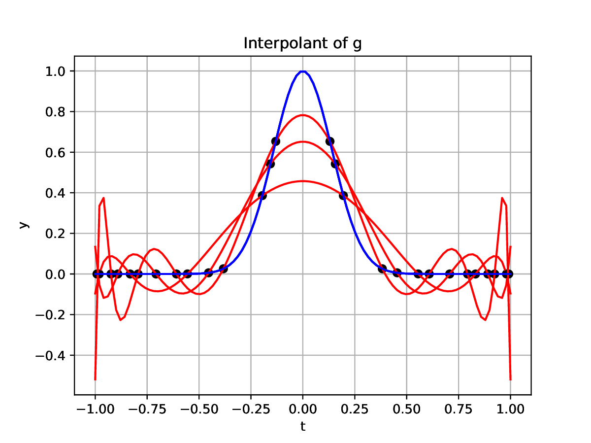
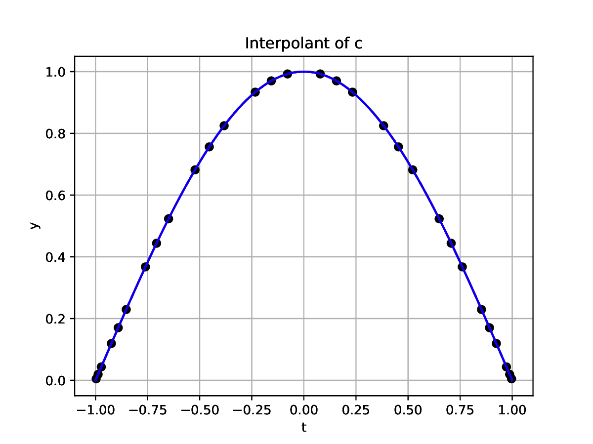
Figure 2. Interpolation results for Chebyshev partitions of $f (t) \in {\cos (π t / 2), 1 / (1 + 25 t^{2}), \exp (- 25 t^{2})}$

∴	function MonomialBasis(t,n) m=size(t)[1]; A=ones(m,1); for j=1:n-1 A = [A t.^j] end return A end;

∴

function plotInterp(a,b,f,Basis,m,n,M,txt)
  data=Csample(a,b,f,m); t=data[1]; y=data[2]
  Data=sample(a,b,f,M); T=Data[1]; Y=Data[2]
  A = Basis(t,n); c = A\y; z = Basis(T,n)*c
  plot(t,y,"ok",T,z,"-r",T,Y,"-b"); grid("on");
  xlabel("t"); ylabel("y");
  title(txt)
end;

∴

$x_{i} = \cos [\frac{2 i - 1}{2 n} π]$ $, i = 1, \dots, n,$

∴	function Csample(a,b,f,m) i = 1:m; θ = (2 .* i .- 1)pi/(2m) ; t = (cos.(θ) .+ 1)*(b-a)/2 .+ a; y = f.(t) return t,y end;

∴	function sample(a,b,f,m) t = LinRange(a,b,m); y = f.(t) return t,y end;

∴	c(t)=cos(pit/2); f(t)=1/(1+25t^2); g(t)=exp(-(5*t)^2);

∴	FigPrefix=homedir()*"/courses/MATH661/homework/H06/";

∴	clf(); plotInterp(-1,1,c,MonomialBasis,10,10,100,"Interpolant of c");

∴	plotInterp(-1,1,c,MonomialBasis,20,20,100,"Interpolant of c");

∴	savefig(FigPrefix*"Fig02a.eps")

∴	clf(); plotInterp(-1,1,f,MonomialBasis,8,8,100,"Interpolant of f");

∴	plotInterp(-1,1,f,MonomialBasis,10,10,100,"Interpolant of f");

∴	plotInterp(-1,1,f,MonomialBasis,12,12,100,"Interpolant of f");

∴	savefig(FigPrefix*"Fig02b.eps")

∴	clf(); plotInterp(-1,1,g,MonomialBasis,8,16,100,"Interpolant of g");

∴	plotInterp(-1,1,g,MonomialBasis,10,20,100,"Interpolant of g");

∴	plotInterp(-1,1,g,MonomialBasis,12,34,100,"Interpolant of g");

∴	savefig(FigPrefix*"Fig02c.eps")

∴

Observations. For both equidistant and Chebyshev sampling interpolation converges with increasing $n$ for $f (t) = \cos (π t / 2)$ . For both other functions the error grows without bound away from the interpolation data points, albeit slower for Chebyshev sampling. This is suggested from the error formula by bounding derivatives and $| w (t) | = | \prod_{i = 0}^{n} (t - x_{i}) | < 2^{n + 1}$ for $t \in [- 1, 1]$ .

$f (t) = \cos (π t / 2)$ , has a readily determined derivative bound $| f^{(n + 1)} (t) | ⩽ {(π / 2)}^{n + 1}$ ,
${lim}_{n \to \infty} {(\frac{π}{2})}^{n + 1} \frac{2^{n + 1}}{(n + 1)!} = 0 .$
$f (t) = 1 / p (t) = 1 / (1 + 25 t^{2}) = 1 / (1 + c t^{2})$ . The first few derivatives are
$f^{'} = - \frac{p^{'}}{p^{2}} = - \frac{50 t}{{(1 + 25 t^{2})}^{2}}, f^{''} = - \frac{p^{''}}{p^{2}} + \frac{2 {(p^{'})}^{2}}{p^{3}} = - \frac{50}{{(1 + 25 t^{2})}^{2}} + \frac{2 {(50 t)}^{2}}{{(1 + 25 t^{2})}^{3}},$ $f^{'''} = \frac{6 p^{'} p^{''}}{p^{3}} - \frac{6 {(p^{'})}^{3}}{p^{4}} = \frac{6 \cdot (50 t) \cdot 50}{{(1 + 25 t^{2})}^{3}} - \frac{6 {(50 t)}^{3}}{{(1 + 25 t^{2})}^{4}},$ $f^{(4)} = \frac{6 {(p^{''})}^{2}}{p^{3}} + \dots$
Notice that $f^{(2 k)} (t)$ has a local extremum at $t = 0$ for which $f^{(2 k + 1)} (0) = 0$ , and
$f^{(2 k)} (0) ∽ 𝒪 (2 k!) c^{k},$
gives a rapidly increasing error bound.
As above, repeated differentiation suggests a rapidly increasing upper bound $f^{(n)} (0) ∽ 𝒪 (2 k!)$ .

2Track 1

For $n = 5$ equidistant sample points, explicitly write the Lagrange and Newton forms of the interpolating polynomial.

Solution 1. Choose $x_{i} = i$ for $i = 0, 1, \dots, 4$ to obtain interpolations of data $𝒟 = {(x_{i}, y_{i}), i = 0, 1, \dots, n - 1}$

ℓ_{0} (t) = \prod_{j = 0, j \neq 0}^{4} \frac{(t - i)}{(j - i)} = \frac{t - 1}{1 - 0} \cdot \frac{t - 2}{2 - 0} \cdot \frac{t - 3}{3 - 0} \cdot \frac{t - 4}{4 - 0}

ℓ_{1} (t) = \prod_{j = 0, j \neq 1}^{4} \frac{(t - i)}{(j - i)} = \frac{t}{0 - 1} \cdot \frac{t - 2}{2 - 1} \cdot \frac{t - 3}{3 - 1} \cdot \frac{t - 4}{4 - 1}

ℓ_{2} (t) = \prod_{j = 0, j \neq 2}^{4} \frac{(t - i)}{(j - i)} = \frac{t - 0}{0 - 2} \cdot \frac{t - 1}{1 - 2} \cdot \frac{t - 3}{3 - 2} \cdot \frac{t - 4}{4 - 2}

ℓ_{3} (t) = \prod_{j = 0, j \neq 3}^{4} \frac{(t - i)}{(j - i)} = \frac{t - 0}{0 - 3} \cdot \frac{t - 1}{1 - 3} \cdot \frac{t - 2}{2 - 3} \cdot \frac{t - 4}{4 - 3}

ℓ_{4} (t) = \prod_{j = 0, j \neq 4}^{4} \frac{(t - i)}{(j - i)} = \frac{t - 0}{0 - 4} \cdot \frac{t - 1}{1 - 4} \cdot \frac{t - 2}{2 - 4} \cdot \frac{t - 3}{3 - 4}

p (t) = \sum_{i = 0}^{4} y_{i} ℓ_{i} (t)

Construct table of divided differenes for Newton form

\begin{array}{lllllll} i & x_{i} & y_{i} & [y_{i}, y_{i - 1}] & [y_{i}, y_{i - 1}, y_{i - 2}] & [y_{i}, y_{i - 1}, y_{i - 2}, y_{i - 3}] & [y_{i}, y_{i - 1}, y_{i - 2}, y_{i - 3}, y_{i - 4}] \\ 0 & 0 & y_{0} & - & - & - & - \\ 1 & 1 & y_{1} & y_{1} - y_{0} & - & - & - \\ 2 & 2 & y_{2} & y_{2} - y_{1} & \frac{1}{2} (y_{2} - 2 y_{1} + y_{0}) & - & - \\ 3 & 3 & y_{3} & y_{3} - y_{2} & \frac{1}{2} (y_{3} - 2 y_{2} + y_{1}) & \frac{1}{6} (y_{3} - 3 y_{2} + 3 y_{1} - y_{0}) & - \\ 4 & 4 & y_{4} & y_{4} - y_{3} & \frac{1}{2} (y_{4} - 2 y_{3} + y_{2}) & \frac{1}{6} (y_{4} - 3 y_{3} + 3 y_{2} - y_{1}) & \frac{1}{24} (y_{4} - 4 y_{3} + 6 y_{2} - 4 y_{1} + y_{0}) \end{array}

leading to

p (t) = y_{0} + (y_{1} - y_{0}) t + \frac{1}{2} (y_{2} - 2 y_{1} + y_{0}) t (t - 1) + \frac{1}{6} (y_{3} - 3 y_{2} + 3 y_{1} - y_{0}) t (t - 1) (t - 2) + \frac{1}{24} (y_{4} - 4 y_{3} + 6 y_{2} - 4 y_{1} + y_{0}) t (t - 1) (t - 2) (t - 3)

3Track 2

Repeat the above convergence study for Hermite interpolation $p_{n} (x_{i}) = f (x_{i})$ , $p_{n}^{'} (x_{i}) = f^{'} (x_{i})$ , $i = 1, 2, \dots, n$ .

Solution. Modify functions from L19 to obtain results in Fig. 3. Overall behavior is as in regular interpolation in function values, but with more accurate results for the Chebyshev points for the Runge function.

$\circ$

Figure 3. Interpolation results for equidistant partitions of $f (t) \in {\cos (π t / 2), 1 / (1 + 25 t^{2}), \exp (- 25 t^{2})}$

∴	function MonomialBasis(t,n) m=size(t)[1]; D0=ones(m,1); D1=zeros(m,1); a=[D0; D1]; A=a; for j=1:2n-1 D0=t.^j; D1=jt.^(j-1); a = [D0; D1] A = [A a] end return A end;

∴

function plotInterp(a,b,f,df,Basis,m,n,M,txt)
  data=sample(a,b,f,df,m); t=data[1]; y=data[2]; yp=data[3];
  Data=sample(a,b,f,df,M); T=Data[1]; Y=Data[2]; Yp=Data[3];
  A = Basis(t,n); a = A\[y; yp]; z = Basis(T,n)*a
  plot(t,y,"ok",T,z[1:M],"-r",T,Y[1:M],"-b"); grid("on");
  xlabel("t"); ylabel("y");
  title(txt)
end;

∴	function sample(a,b,f,df,m) t = LinRange(a,b,m); y = f.(t); yp = df.(t) return t,y,yp end;

∴	c(t)=cos(pit/2); f(t)=1/(1+25t^2); g(t)=exp(-(5*t)^2);

∴	dc(t)=-pi/2sin(pit/2); df(t)=-50t/(1+25t^2)^2; dg(t)=-50texp(-(5*t)^2);

∴	FigPrefix=homedir()*"/courses/MATH661/homework/H06/";

∴	clf(); plotInterp(-1,1,c,dc,MonomialBasis,10,10,100,"Interpolant of c");

∴	plotInterp(-1,1,c,dc,MonomialBasis,20,20,100,"Interpolant of c");

∴	savefig(FigPrefix*"Fig03a.eps")

∴	clf(); plotInterp(-1,1,f,df,MonomialBasis,8,8,100,"Interpolant of f");

∴	plotInterp(-1,1,f,df,MonomialBasis,10,10,100,"Interpolant of f");

∴	plotInterp(-1,1,f,df,MonomialBasis,12,12,100,"Interpolant of f");

∴	savefig(FigPrefix*"Fig03b.eps")

∴	clf(); plotInterp(-1,1,g,dg,MonomialBasis,8,8,100,"Interpolant of g");

∴	plotInterp(-1,1,g,dg,MonomialBasis,10,10,100,"Interpolant of g");

∴	plotInterp(-1,1,g,dg,MonomialBasis,12,12,100,"Interpolant of g");

∴	savefig(FigPrefix*"Fig03c.eps")

∴

$\circ$

Figure 4. Interpolation results for Chebyshev partitions of $f (t) \in {\cos (π t / 2), 1 / (1 + 25 t^{2}), \exp (- 25 t^{2})}$

∴	function MonomialBasis(t,n) m=size(t)[1]; D0=ones(m,1); D1=zeros(m,1); a=[D0; D1]; A=a; for j=1:2n-1 D0=t.^j; D1=jt.^(j-1); a = [D0; D1] A = [A a] end return A end;

∴

function plotInterp(a,b,f,df,Basis,m,n,M,txt)
  data=Csample(a,b,f,df,m); t=data[1]; y=data[2]; yp=data[3];
  Data=sample(a,b,f,df,M); T=Data[1]; Y=Data[2]; Yp=Data[3];
  A = Basis(t,n); a = A\[y; yp]; z = Basis(T,n)*a
  plot(t,y,"ok",T,z[1:M],"-r",T,Y[1:M],"-b"); grid("on");
  xlabel("t"); ylabel("y");
  title(txt)
end;

∴

$x_{i} = \cos [\frac{2 i - 1}{2 n} π]$ $, i = 1, \dots, n,$

∴	function Csample(a,b,f,df,m) i = 1:m; θ = (2 .* i .- 1)pi/(2m) ; t = (cos.(θ) .+ 1)*(b-a)/2 .+ a; y = f.(t); yp = df.(t) return t,y,yp end;

∴	function sample(a,b,f,df,m) t = LinRange(a,b,m); y = f.(t); yp = df.(t) return t,y,yp end;

∴	c(t)=cos(pit/2); f(t)=1/(1+25t^2); g(t)=exp(-(5*t)^2);

∴	dc(t)=-pi/2sin(pit/2); df(t)=-50t/(1+25t^2)^2; dg(t)=-50texp(-(5*t)^2);

∴	FigPrefix=homedir()*"/courses/MATH661/homework/H06/";

∴	clf(); plotInterp(-1,1,c,dc,MonomialBasis,10,10,100,"Interpolant of c");

∴	plotInterp(-1,1,c,dc,MonomialBasis,20,20,100,"Interpolant of c");

∴	savefig(FigPrefix*"Fig04a.eps")

∴	clf(); plotInterp(-1,1,f,df,MonomialBasis,8,8,100,"Interpolant of f");

∴	plotInterp(-1,1,f,df,MonomialBasis,10,10,100,"Interpolant of f");

∴	plotInterp(-1,1,f,df,MonomialBasis,12,12,100,"Interpolant of f");

∴	savefig(FigPrefix*"Fig04b.eps")

∴	clf(); plotInterp(-1,1,g,dg,MonomialBasis,8,16,100,"Interpolant of g");

∴	plotInterp(-1,1,g,dg,MonomialBasis,10,20,100,"Interpolant of g");

∴	plotInterp(-1,1,g,dg,MonomialBasis,12,34,100,"Interpolant of g");

∴	savefig(FigPrefix*"Fig04c.eps")